Method of Weighted Residuals
Approximate solutions of differential equations satisfy only part of the conditions of the problem: the differential equation may be satisfied only at a few positions, rather than at each point. The approximate solution is expanded in a set of known basis functions with arbitrary parameters. In the Method of Weighted Residuals (MWR) one works directly with the differential equation and boundary conditions to choose the parameters in the approximation. A first approximation may be sufficient, and its validity is assessed using our intuition and experience. More commonly today, though, a sequence of approximations is calculated to converge to the solution.
The Method of Weighted Residuals (MWR) actually encompasses several methods: collocation, Galerkin, integral, least squares, etc. The integral method has been widely used in fluid mechanics, the collocation method has been widely used in chemical engineering, and the Galerkin method forms the basis for the finite element method so prevalent today. An alternative to the Method of Weighted Residuals is the variational method (link). This method requires that the problem be derivable from a variational principle, and then the parameters in the expansion are found by making a variational integral stationary, and in some cases a minimum. A summary of the early history of the methods making up MWR is available (link - p. 9-11 + Petrov).
We apply the Method of Weighted Residuals in five steps:
1. Expand the unknown solution in a set of basis functions, with unknown coefficients or parameters; this is called the trial solution.
2. Make the trial solution satisfy the boundary conditions (usually).
3. Define the residual.
4. Set the weighted residual to zero and solve the equations.
5. Examine the error by constructing successive approximations, and show convergence as the number of basis functions increases.
Let us do this first for a general equation, and then apply the method to a specific example. Consider the problem
![]()
where L is a linear operator defined on some region of space. (The same ideas apply to nonlinear equations, and time-dependent problems, but the algebra is more extensive.) Expand the unknown solution in a series
![]()
where the functions y0 and yi(x) are known functions chosen by us. This expansion was written as the sum of a function which satisfies the non-homogeneous boundary conditions (the right-hand side is not zero), and a linear combination of {yi(x)}, each of which satisfy the homogeneous boundary conditions (the right-hand side is zero).
![]()
Then the trial function satisfies the boundary conditions for any choice of the parameters {ai}. We have completed the first two steps in MWR. Next we rearrange the differential equation so that the right-hand side is zero.
![]()
Substitute the trial function into the differential equation to form the residual (step 3).
![]()
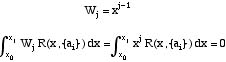
Multiply the residual by a weighting function (defined below) and integrate over the domain to form the weighted residual, and make the weighted residual zero.
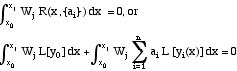
![]()
We set the weighted residual to zero since we want the differential equation satisfied, in which case the residual is zero for all x; the trial function already satisfies the boundary conditions. Since the weighted residual contains some unknown parameters, {ai}, we use as many weighting functions as we have parameters (generally). We thus have formed a set of linear equations for the parameters. We solve the equations (step 4) to find the approximate solution. To determine how accurate the solution is, we repeat the process using more terms in the expansion (more basis functions), giving a larger set of nonlinear equations; we continue that process until our accuracy needs are met.
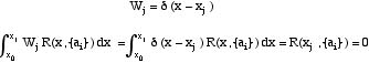
There are a variety of choices for the weighting function, and each one gives rise to a method with a different name. In the collocation method, we use a Dirac delta function; then the weighted residual corresponds to setting the residual equal to zero at the singularity of the Dirac delta function.
In the least squares method, we use as weighting function a derivative of the residual.
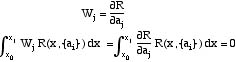
If we write the mean square residual
![]()
and minimize it with respect to the parameters we get the least squares method.
In the integral method, we integrate over part of the domain.
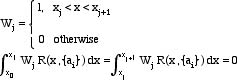
In boundary layer flows, for example, we might integrate over the whole boundary layer (for the first approximation) and then over parts of the boundary layer (for higher approximations).
In the method of moments, we multiply the residual by a variable (like x in a boundary value problem) and integrate over the domain.,
In the Petrov-Galerkin method, we multiply by each member of a new set of functions, sometimes called test functions. These need not be the same as the basis functions in the trial solution.
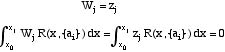
In the Galerkin method, which was derived first historically, the test functions are the same functions used in the basis set.
![]()
As an aside, when a variational principle exists for the problem, the Galerkin method and variational method will be the same, if applied appropriately.
Now why would any of this work? The chief reason is that if a function is made orthogonal to every member of a complete set of functions, that function is zero. Here the function is the residual, and the complete set of functions are the basis functions (for the Galerkin method), the powers of x (for the integral method), etc. More detail is available (link).
See an example application.