Figures showing CARS data
- Bathymetry
- Bathymetry of the SW Pacific
- Bathymetry across the S Pacific
- Bathymetry near the Tuamotus
- CARS bottom depths near NC Bottom for shallow DH Detail
- Bathymetry near PNG: etopo2 etopo20 etopo20 on CARS grid Bottom for DH2000 CARS bottom depths
- Main bathymetry page
- Maps of velocity and transport (also see "SEC bifurcation and WBC work" below (section 4))
- Geostrophic transport function:
- Contours: Shaded (v2) Colored contours
- Vectors: Vectors With bathymetry Correct aspect ratio Extend to EAC Add bathymetry NC detail
- Zonal component of transport Another version with overlaid DH (unlabeled for ppt)
- Transport magnitude (overlay vectors)
- Compare Ridgway/Dunn Fig 3 Extra contours
- Transport above and below 500m Detail near NC
- Recalculate transport relative to 2000m:
- Depths shallower than 2000m
- Velocities: u_g at 1200m relative to 2000m
DH and u_g at the surface Zonal component Meridional component
- 0-2000m transport
- 0-1200m transport (2000m ref level)
- 1200m-2000m transport
- Zonal component of transport: 0-2000m 1200m-2000m 0-1200m (2000m ref level) 0-1200m (1200m ref level)
- Meridional component: 0-2000m transport 1200m-2000m transport
- Surface velocity rel 2km (NC detail)
- Compare CARS, BMRC and Levitus transport (NC-Vanuatu detail)
- Maps of DH and u_g (also see some 2000m figs above):
- Surface: SW Pacific NC detail Zonal component (50m) (Overlay wind)
- 100m: SW Pacific NC detail Zonal component (150m)
- 200m: SW Pacific NC detail Zonal component (250m)
- 300m: SW Pacific NC detail Zonal component (350m)
- 400m: SW Pacific NC detail Zonal component (450m)
- 500m: SW Pacific NC detail Zonal component
- 600m: SW Pacific Zonal component
- 750m: SW Pacific NC detail
- Transport Surface u_g vs transport
- Maps of isotherm depths:
- Z25: Z25
- Z25: Z20
- Z25: Z15
- Z25: Z12
- Z25: Z10
- Z25: Z8
- Z25: Z5
- Quantities on isopycnals (35°S-10°S; also see sections 4.4,5,8 below):
- Sigmat=24: Streamfunction u Depth
- Sigmat=24.5: Streamfunction u v Salinity
- Sigmat=25: Streamfunction u Depth Salinity
- Sigmat=25.5: Streamfunction u v
- Sigmat=26: Streamfunction u v Depth
- Sigmat=26.5: Streamfunction u v Salinity
- Sigmat=27: Streamfunction u Depth Salinity
- Basinwide isopycnal depths: Sigma 27.0 27.2
- Quantities along jet cores:
- Depth: Tube Vector
- Speed: Tube Vector
- Temperature: Tube Vector
- Salinity: Tube Vector
- Density: Tube Vector
- Westward transport Overlay vectors
- Meridional sections
- Meridional sections of u_g (overlay sigma-t)
- Meridional section of u_g (overlay T) at 170°E-180°
- Stretched full-depth sections (made for Jay):
160°E
180°
160°W
- ug and overlay T at 160°W, 50°S-5°S
- Work on the SEC bifurcation region and the NGCC
(Much of this work is for comparisons with the ORCA model)
(Also see "Quantities on isopycnals" in section 2f above)
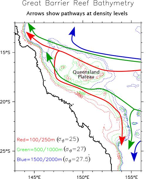
- Maps of the GBR bathymetry: Times Atlas (scanned) etopo5
- Schematic currents over bathymetry: JPG PDF
- Maps of DH and u_g by depth: Vectors only With DH contours Show bifurcation
- Bifurcation latitude as a function of depth Overlay estimates from density
- Maps of sigma-theta surfaces: 27.5-27-26.5-26 25.5-25-24.5-24 (see also Figs 2.f above)
- Maps of MSF and u_g by density: 27.5-27-26.5-26 25.5-25-24.5-24 (pdf files; 35°S-10°S)
- DH and winds near the coast
- Finding the bifurcation at the coastal gridpoints:
- Rel 2000m, one-sided differencing
- Rel 2000m, centered differencing
- Rel 1000m, from annual cycle
- Rel 1000m, annual cycle at sfc
- Vectors by level:
- Vectors Overlay dynamic ht
- Salinity on corresponding levels Salinity on isopycnals
- Using T-S properties to trace the flow into the NGCC:
- Salinity on isotherms (21,22,23,24) Depths of isotherms Isopycnals on isotherms
- Salinity on isopycnals:
(23.5,24,24.5,25)
(24,24.4,24.8,25.2)
(25.4,25.6,25.8,26)
(26.2,26.4,26.6,26.8)
(27,27.1,27.2,27.3)
- Salinity along the coast of Australia
- Maps of salinity and flow on sigma-theta=24.5: Salinity
Streamline overlays: White White+vectors Color-coded Fewer
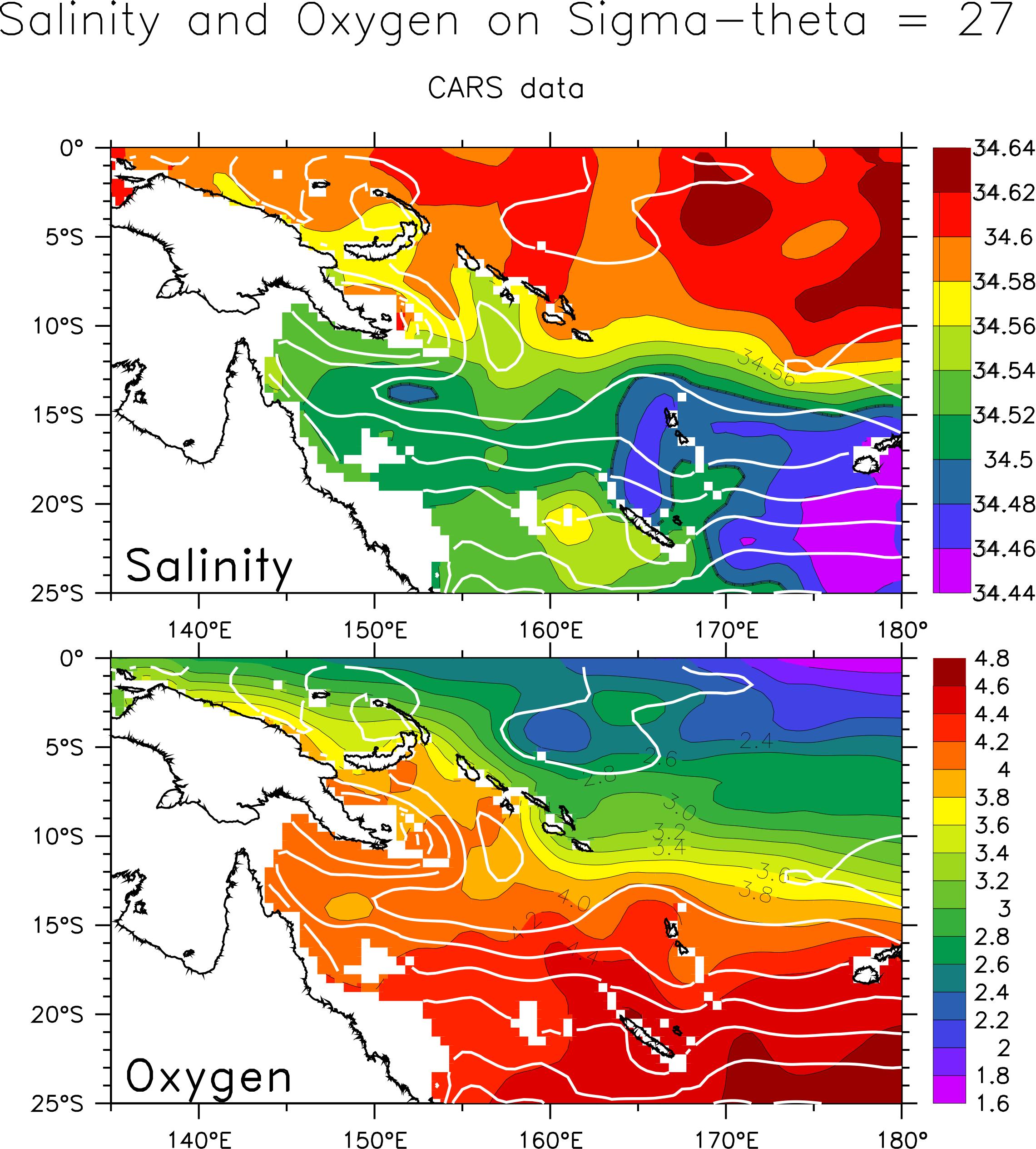
- Salinity and oxygen on sigma 27
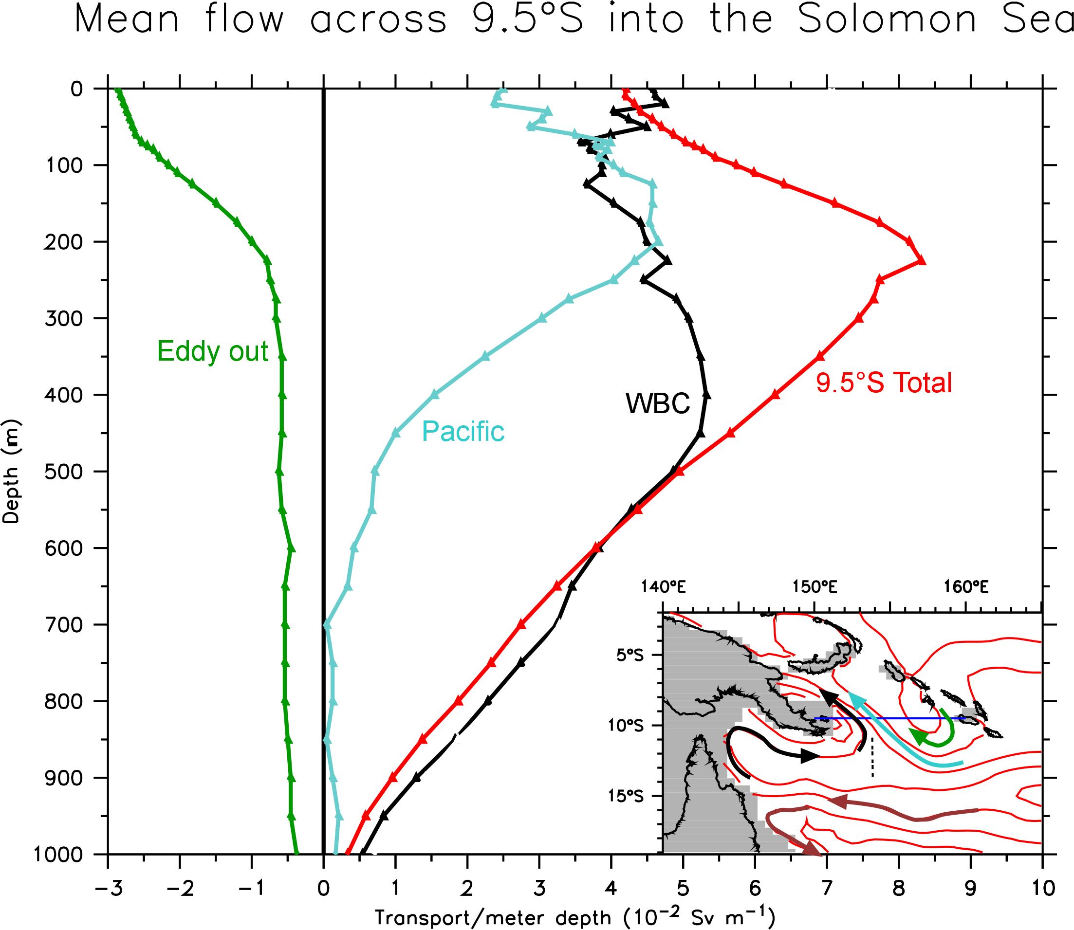
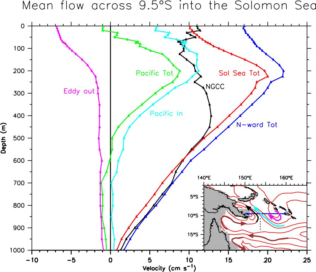
- Estimates of the transport into the Solomon Sea:
- Transports across 9.5°S: NGCC, Pacific In, Eddy out, Totals Downward integral of transports
From Cairns talk: Talk figure All profiles
- NGCC, NQC, Net Pacific
- NQC estimates: Transport/meter Downward integral
- Checking (DH across the NQC): 11.5°S 12°S 12.5°S 13°S
- 3-panel Solomon Sea transport (Cairns talk) (pdf file)
- Estimating the bifurcation according to Firing et al (1999) principle:
"... an inflow to the boundary current will split,
with fraction (y-y_s)/(y_n-y_s) going north,
and the remainder going south"
Use ORCA zonal current at 163°E as inflow to the WB.
Do calculation on density levels. [Note that this work was done in the cars directory]
Many figures from CARS in this section: Find them on the ORCA page, section 8g
- Unsorted files made for Cairns
Solomon Sea transport estimates and a few other things.
- Zonal sections of v_g:
- 5°S
- 8°S
- 12°S
- 15°S
- 20°S
- 25°S
- 30°S
- Zonal sections of v_g (eddy tilt): 24°S 23°S 22°S 21°S 18°S
- Sections across the permanent (?) eddy at 165°E, 24°S: (165°E,y,z) (166°E,y,z) (x,24°S,z)
- PV maps and sections:
- Meridional sections vs theta: 175°W 175°E 165°E 160°E
- Meridional sections vs z, overlay u: 175°W 172°E 161°E
- Maps on sigma-theta: 25.5 26 26.5 27
Overlay u_g vectors: 26.5 26.8
Sigma-theta level where Q=10e-10
- PV maps from CARS09:
25.0 25.5 26.0 26.5 26.7 27.0 27.2
- DH and u_g maps near Fiji (compare Morris, Roemmich and Cornuelle 96 JPO):
Surface
50m
100m
150m
200m
300m
400m
500m
600m
750m
1000m
- Annual cycle:
- CARS annual cycle transport variance ellipses: V1 To 8°S Omit mean vectors To 160°W
Omit vectors
- Transport harmonic along variance ellipses
- Jets:
- mean u_g(y,z) along 160°E: Rel 1000m Rel 2000m
- Relation between DH variability and sfc u_g
- Jets time series: Surface u_g at the jet cores Transport time series
Compare ORCA Rossby solution Combined CARS, Rossby model and ORCA transport at 160°E
- CARS and Rossby model transport at 160°E (y,t)
- Some results from the WOCE P11S section along 155°E:
- Track map 1 Stations used here
- (y,z) sections: Temperature Salinity Oxygen
- (y,z) sections of u_g: Whole section To 30°S Compare CARS
- P11 and CARS transport integrated along the track
- ORCA along P11S comparisons: Mean U U@iin, Mean/Jun/Dec U@iin, seasonal
- Combined zonal transport comparison P11S, CARS, ORCA
Return to main page
Other pages: