4 Estimating the Heritability of Spot Count

Following the instructions in the previous chapter, collect data on at least 20 families of ladybugs. The more families you include, the more accurate your estimate of the heritability will be.

As soon as you have begun entering data for the third family, the graph in the Analyze Families tab will show the best-fit line through your data points.

The best-fit line, in blue, reveals the extent to which the variation among the parents has been transmitted to the offspring. (You will want a bigger sample size than is shown here.)

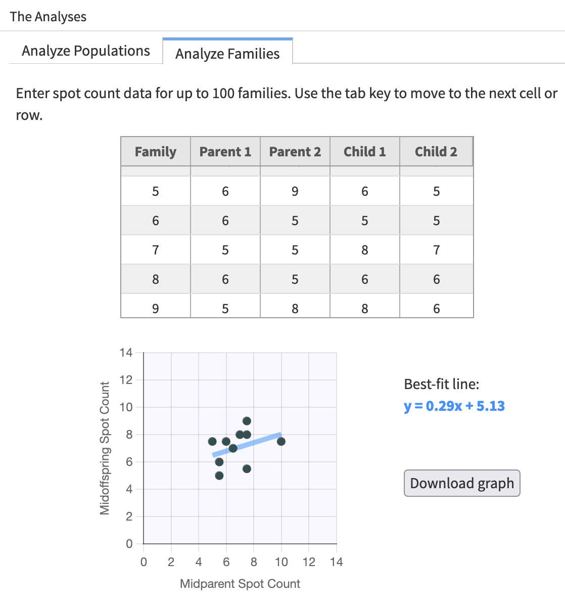
The line will update as you add more data. The equation for the line, in slope-intercept form, appears to the right of the graph. The slope is the number in front of “x”. The equation for the line is calculated using least-squares linear regression—the standard method for finding best-fit lines. If that last sentence doesn’t mean anything to you, don’t worry about it!

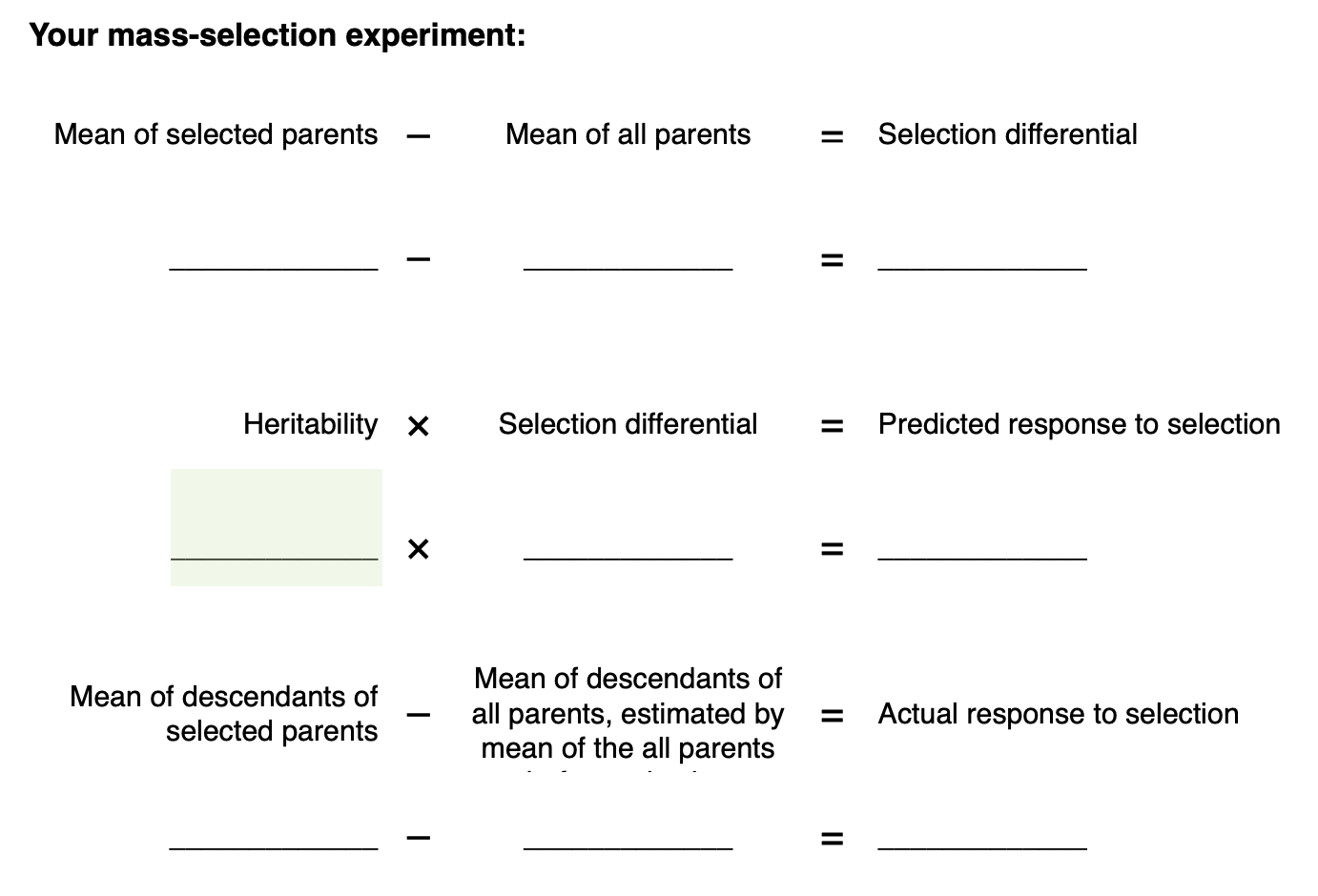
We can take the slope of the best-fit line for a parent-offspring regression—like the one you have just produced—as an estimate of the heritability of the trait in question. In principle, this number falls somewhere between 0 and 1. It tells us how much of the variation among the parents is due to differences in the genes they carry (as opposed to random environmental effects).

Before proceeding, be sure to record your estimate of the heritability of spot count in the Bugsville worksheet:

Write your estimate of the heritability of spot count in the highlighted space.