Transfer
Function
Frequency
Response
Lesson 10- Non-linear Material Behavior
Background
The analysis employed by DR. Layer required an appropriate
idealization of the stress-strain relationship. Two such idealizations
were used- linearly elastic and bilinear models. The linearly elastic
model assumes a constant variation of stress and strain according to Hooke's
law with no permanent deformations after the applied stresses is removed.
This holds true until the yield point followed by an unrestricted plastic
strain after yield.
A nonlinear (varying stress- strain relationship) model may also be used
for soils from the beginning of loading. For our analysis this is implemented
as a bilinear model with the following characteristics
1. Strain E1
2. An initial shear modulus G1 until a limiting strain E1
3. A Shear modulus G2 after the strain E1
When the direction of the applied loading is reversed, behavior is again determined by the modulus G1 until a strain change of 2E1 is obtained and then the modulus G2 takes control of the behavior. This pattern is continuously repeated. An option to include strain hardening is included which provides the opportunity to play with the possibility of including permanent deformation.
BACK TO TOP
Objective
After this exercise you will have a better understanding of two idealized models used to obtain stress-strain curves in practice.Things to Do
- Open the Dr. Layer program. By default we get twelve layers. The top
six layers are hardwired into the system with a velocity specified as
very fast. The bottom six layers are hardwired with a velocity of very
slow.
- Select all (Edit menu) the layers to all have very slow values or
any combination you desire.
- On the menu listings choose options and material model by default
we have a linearly elastic model.
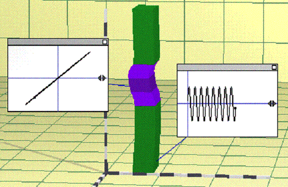
- Push the ctrl key and apply the label tool at the mid layer level.
You should get a stress-strain plot with origin in the middle of the
plot area. A combination of different layer types can give you plots
like that shown below in Fig. 8.1

- Return to zero time by pushing bottom left button and try many combinations
as possible varying as many parameters as you desire.
- Next we will change the to a bilinear, medium stressed and strain
hardened material model. This can be achieved in the options menu and
material model. To get a reasonable visual effect you need to increase
the amplitude to its maximum value. Also apply a very low damping value
to the layers and with strain hardening you will obtain the permanent
deformation shown below.

BACK TO TOP
Observation
The material models employed show marked differences when turned on. The stress-strain curves obtained are different for each case. Turning on strain hardening causes permanent irreversible deformation with a decrease in load applied.On Your Own
- Obtain stress-strain plots that will display a bilinear relationship (seen as multiple slant lines displaced from the origin.
BACK TO TOP
Last
Updated:
12/27/00
Contact us at: parduino@u.washington.edu