Orthogonal Polynomials for Interpolation

Orthogonal polynomials are defined in such a way that the interpolation gives the best fit over the entire region. We require the polynomials to be orthogonal to each other; this is only necessary to improve the accurcy when high-order polynomials are used. Thus, we take P_m(x) to be orthogonal to P_k(x) for all k=0,...,m-1.

The orthogonality includes a non-negative weight function, W(x)0 for all axb. This procedure specifies the set of polynomials to within multiplicative constants, which can be set by either requiring the leading coefficient to be one or by requiring the norm to be one.

The polynomial P_m(x) has m roots in the closed interval a to b.

The polynomial

minimizes

when

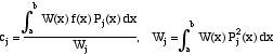
Note that each c_j is independent of m, the number of terms retained in the series. The minimum value of I is

Such functions are useful for continuous data, i.e. when f(x) is known for all x.

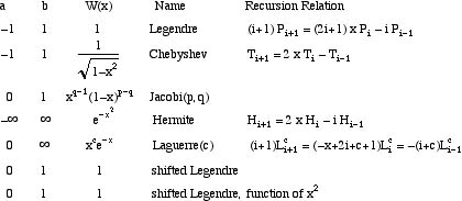
Typical polynomials are given in the Table I. Chebyshev polynomials are used in spectral methods (link). The last few entries are widely used in the orthogonal collocation method within chemical engineering.

Table I. Orthogonal Polynomials

[Courant and Hilbert, 1953], [Press, et al.,1986]

The last entry is defined by

where a=1, 2, or 3 is for planar, cylindrical, or spherical geometry. These functions are useful if it can be proven that the solution is an even function of x.

Other interpolation schemes are: global polynomials as powers of x that go through a fixed number of points; rational polynomials that are ratios of polynomials; piecewise polynomials derived with forward differences (points to the right) and backward differences (points to the left); splines; and finite elements.

Take Home Message: Orthogonal Polynomials are useful for minimizing the error caused by interpolation, but the function to be interpolated must be known throughout the domain. The use of orthogonal polynomials, rather than just powers of x, is necessary when the degree of polynomial is high.