Finite Element Interpolation

Overview of Finite Element Interpolation

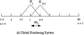
The finite element method can be used for piecewise approximations [Finlayson, 1980]. Divide the domain a < x < b into elements as shown in Figure 1.

'

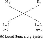
Figure1. Galerkin finite element method ­ linear functions

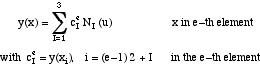
Each function N_i (x) is zero at all nodes except x_i; N_i (x_i) = 1. Thus, the approximation is

where c_i = y (x_i). It is convenient to define the trial functions within an element using new coordinates.

The x_i need not be the same from element to element. The trial functions are defined as N_i(x) in the global coordinate system and N_I(u) in the local coordinate system (which also requires specification of the element). For x_i < x < x_i+1

since all the other trial functions are zero there. Thus, also

We write

Thus we rewrite the expansion as

and c_i = c_I^e within the element e. Thus, given a set of points (x_i, y_i ) a finite element approximation can be made to go through them.

It is also possible to use quadratic approximations within the element. See Figure 2.

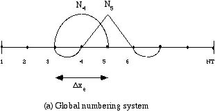
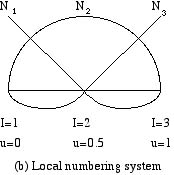
Figure 2. Finite Element Approximation - Quadratic Elements

Now the trial functions are

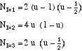
The approximation going through an odd number of points ( x_i, y_i ) is then

Other interpolation schemes are: global polynomials as powers of x that go through a fixed number of points; orthogonal polynomials of x that give a best fit; rational polynomials that are ratios of polynomials; piecewise polynomials derived with forward differences (points to the right) and backward differences (points to the left); and splines.