7 Using an Analytical Model
In the previous section, you predicted the direction and—perhaps, roughly—the speed at which allele frequencies change in your virtual duck population. In this section, we will look at how we can use an analytical model to make a precise quantitative prediction.
We will go through an example, using a different population of imaginary birds, showing how we can use the arithmetic of the Hardy-Weinberg Equilibrium Principle to make a precise prediction of how a population will evolve.
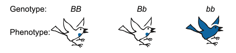
Consider an imaginary songbird population in which, as in our ducks, color is determined by a single gene with two alleles:
We will follow the songbird population around its life cycle, tracking the frequencies of alleles B and b. The life cycle starts with eggs and sperm, collectively referred to as the “gene pool.” The eggs and sperm combine to make zygotes. The zygotes develop into chicks. The chicks—some of them, anyway—grow up to become adults. The cycle is complete when the surviving adult birds make eggs and sperm as they prepare to reproduce:
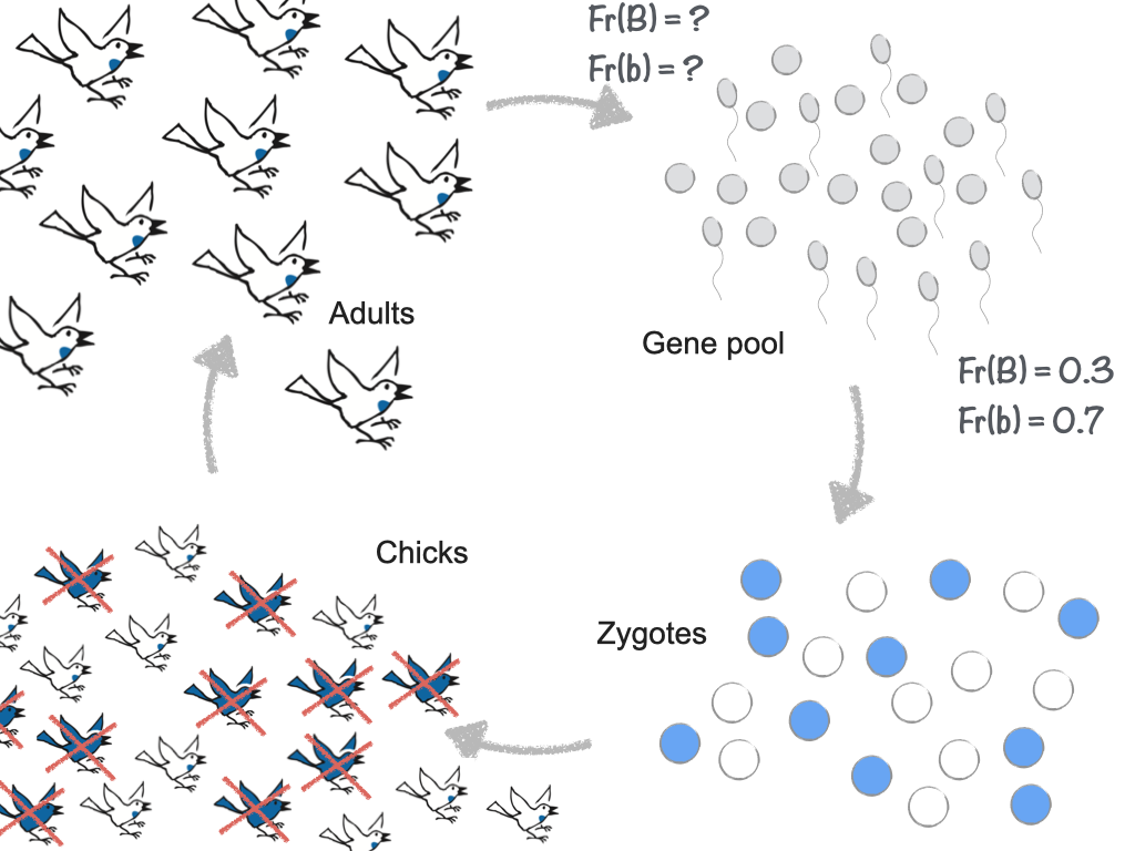
As shown in the diagram, we will imagine that among the eggs and sperm in the gene pool, the frequency of allele B is 30% and the frequency of allele b is 70%. (These numbers are arbitrary. We can work with any frequencies, so long as they add up to 1.)
When the eggs and sperm combine to make zygotes, the zygotes will come in three possible genotypes: BB, Bb, and bb. We need to know the frequencies, which we can calculate with a population Punnett square:
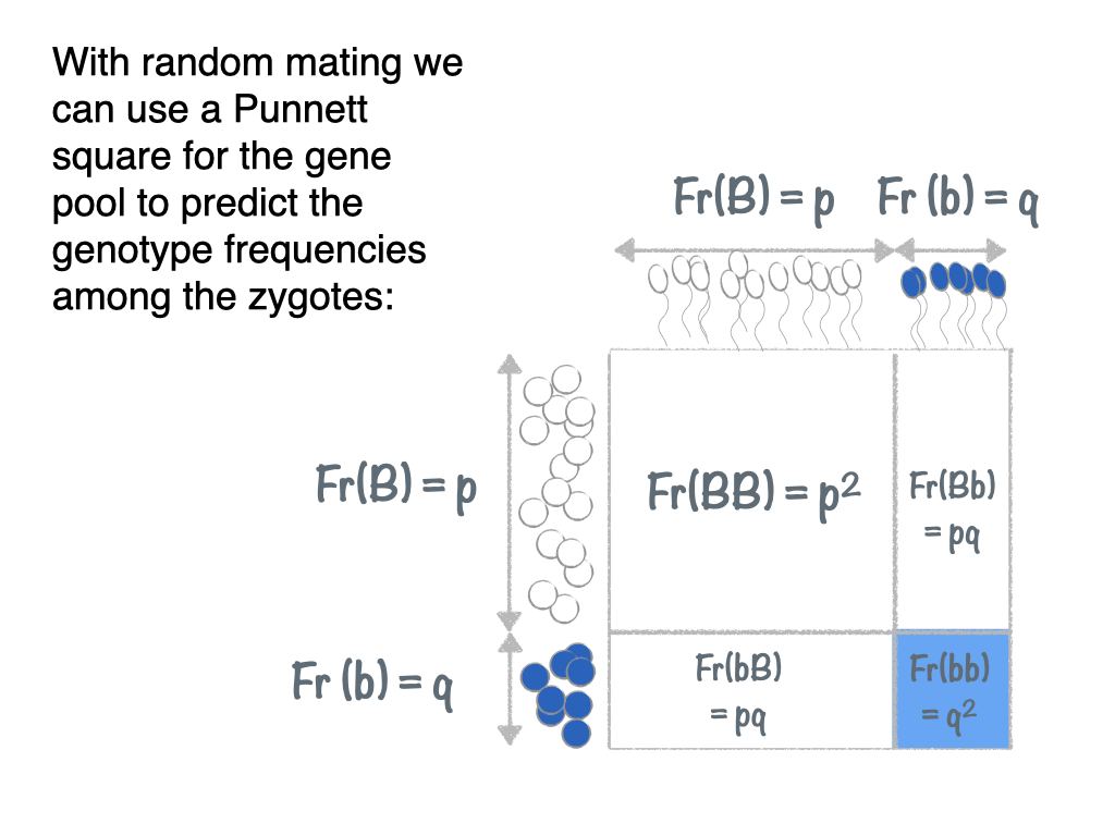
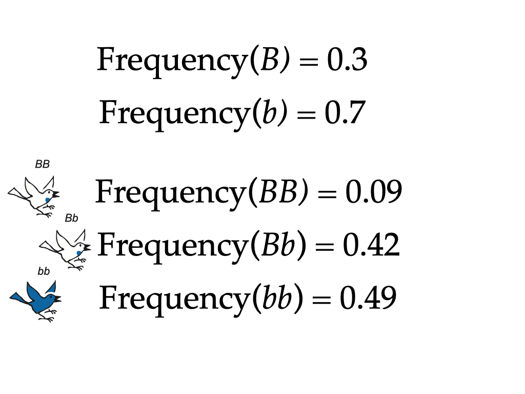
The population Punnett square in the illustration is generic. To apply it to our particular case, we just need to recognize that for us p = 0.3 and q = 0.7. Thus, we have:
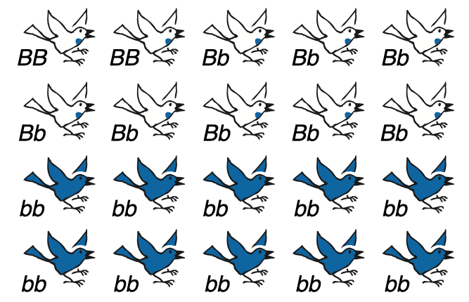
As indicated in the illustration, we will imagine that all the zygotes develop into chicks. At this point, it’s easier (for the author’s brain, anyway) to think about whole numbers than about frequencies. So imagine that we have a (small!) population of just 20 chicks. Using the frequencies we just calculated, and rounding to the nearest whole chick, we have:

Here they are, lined up in rows:
If you look back at the life cycle diagram, you’ll find all 20 chicks at lower left.
Now we imagine that—as with our ducks—the young birds in our population are vulnerable to predation in a way that depends on color. To keep our example simple, we will let all the blue chicks get eaten by cats:
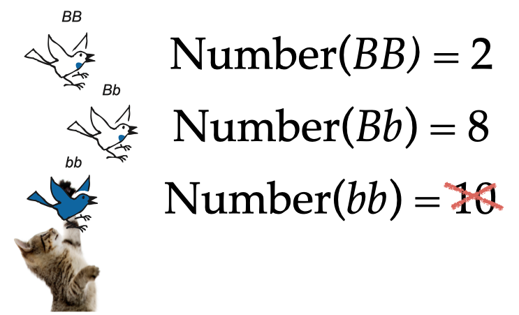
Finally, we let the 10 survivors make gametes to contribute to a new gene pool. What are the new frequencies of alleles B and b?
Calculating the allele frequencies just requires a little more arithmetic. This table shows one method:
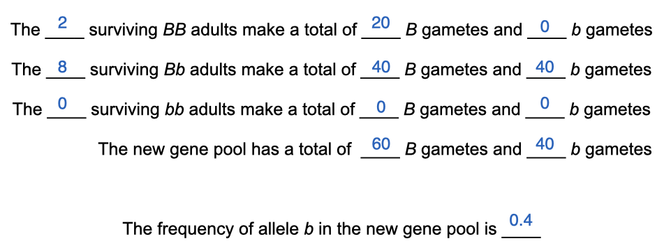
We have let each individual contribute exactly 10 gametes. (Any number will do, but 10 is easy to multiply.) All the gametes made by BB adults carry allele B. Half the gametes made by Bb adults carry B and half carry b. We total the columns for B and b, then calculate the new frequency. Allele b has fallen, in a single generation, from a frequency of 0.7 to a frequency of 0.4.
I made a few delibarate choices that made this example relatively simple. But if you’re willing to do the arithmetic carefully, you can work with any allele frequencies and any survival rates for the three gene genotypes.