One-dimensional Multigrid
Here we consider the following problem from mmf/math/multigrid/notes/multigrid_notes.py:
| Problem(*varargin, **kwargs) | Representation of the following linear problem for use with a one-dimensional multigrid method. |
| MultigridBase(*varargin, **kwargs) | Common base for MultigridNeumann and MultigridPeriodic. |
| MultigridNeumann(*varargin, **kwargs) | Multigrid class for use with Neumann boundary conditions. The interpolation and restriction operators here are: |
| MultigridPeriodic(*varargin, **kwargs) | Multigrid class for use with Periodic boundary conditions. The interpolation and restriction operators here are: |
- class mmf.math.multigrid.notes.multigrid_notes.Problem(*varargin, **kwargs)[source]
Representation of the following linear problem for use with a one-dimensional multigrid method. We provided the following problem:
Problem(a=5,
        periodic=True,
        prob=0)
![\begin{aligned}
-f''(x) &= a\pi^2\left[\cos(\pi x)-a\sin^2(\pi x)\right]
e^{a(\cos\pi x -1)}, \\
-f''(x) + a^2\pi^2\sin^2(\pi x)f(x) &=
a\pi^2\cos(\pi x)e^{a(\cos\pi x -1)}, \\
-f''(x) - a\pi^2\cos(\pi x)f(x) &=
-a^2\pi^2\sin^2(\pi x)e^{a(\cos\pi x -1)}, \\
f(x) &= e^{a(\cos\pi x - 1)}.
\end{aligned}](../_images/math/9376c60bb19550360cfb1946c6d78598411576e3.png)
This can also be written as a non-linear equation:
![-f''(x) = \pi^2\left[\ln f + a - a^2\sin^2(\pi x)\right]f](../_images/math/10dda5e0e14f807d63dc12f4fffb003e465055cc.png)
We may also write this as a set of coupled equations in a few ways, including:
![\begin{aligned}
- f''(x) &= a\pi^2[g - a(1-g^2)]f, \\
- g''(x) &= \pi^2 g = \pi^2 (a^{-1}\ln f + 1)
\end{aligned}](../_images/math/e265765c1de6a4ff094e6d63812eac0c3768488c.png)
This gives rise to the following systems for the Jacobian:
![G_3(f, g) = \begin{pmatrix}
- f''(x) - a\pi^2[g - a(1-g^2)]f, \\
- g''(x) - \pi^2 g
\end{pmatrix}, \qquad
J_3 = -\diff[2]{}{x} + \begin{pmatrix}
- a\pi^2[g - a(1-g^2)] & - a\pi^2[1 + 2g]f\\
0 & - \pi^2
\end{pmatrix}.](../_images/math/855a7a62a68dcac08e16fdbd30743650feb887b1.png)
![G_4(f, g) = \begin{pmatrix}
- f''(x) - a\pi^2[g - a(1-g^2)]f, \\
- g''(x) - \pi^2 (a^{-1}\ln f + 1)
\end{pmatrix}, \qquad
J_4 = -\diff[2]{}{x} + \begin{pmatrix}
- a\pi^2[g - a(1-g^2)] & - a\pi^2[1 + 2g]f\\
- \pi^2 a^{-1}/f & 0
\end{pmatrix}.](../_images/math/3aa0846fdb098a25c214b3eaef98d6c2b0b162a7.png)
Attributes
Discretization
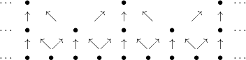
We ignore the boundary conditions for now. In the interior we use the standard 3-point stencil to represent the Laplacian on the interior:
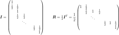
with the interpolation and restriction operators
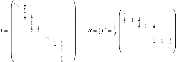
corresponding to the following grid refinements:
These preserve the Galerkin conditions that the restriction and
interpolation operators are transposes and that  . Performing a Fourier analysis, we find
that plane wave eigenvectors
. Performing a Fourier analysis, we find
that plane wave eigenvectors  have eigenvalues

Boundary conditions
One of the challenges is to formulate the boundary conditions in such
a way that the Galerkin conditions are satisfied, i.e. that  and that
  has at least the same
sparsity structure as
has at least the same
sparsity structure as  .
.
It is probably also desirable that the operators preserve their
idempotency for constant functions. Where this is not
possible, one should prefer the property for the interpolation operator
 (this has not been tested here however).
Furthermore, to implement the boundary conditions, it is desirable if the operators can be formulated in such a was as to be implementable by a simple stencil acting on an augmented array. The exclusive Neumann condition has this property where as the inclusive version does not (requiring also modification of the values of the boundary points).
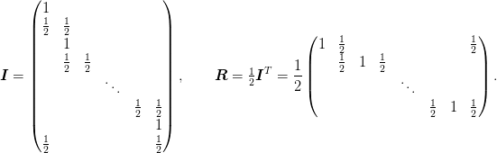
Neumann Boundary Conditions
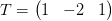
We first consider pure Neumann boundary conditions. We would like to keep the difference operator symmetric (so that eigenvalues are guaranteed to be real for example), which restricts the form of the operator to
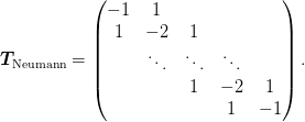
This can be represented by the stencil ![[1, -2, 1]](../_images/math/d5cf7ed159d95f04bbfdf93414a8ab85e2935ebd.png) on the augmented
array
on the augmented
array ![[a,b,\cdots x,y] \rightarrow [a,a,b,\cdots, x,y,y]](../_images/math/cbd4820e19065cda450f3d84ac05e49c4a1b76c8.png) . This is
both symmetric and satisfies the charge neutrality condition. Its
structure is preserved by the interpolation and restriction operators:
. This is
both symmetric and satisfies the charge neutrality condition. Its
structure is preserved by the interpolation and restriction operators:
Note that the restriction operator does preserve constant functions at
the endpoints, but the interpolation operator does. The number of
lattice points is  .
.
There are two interpretations:
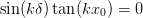
As a straightforward finite-difference operator. In this case, we can inspect the desired eigenvectors of the form
 . Applying this matrix and using the eigenvalue equation
we find the consistency condition:
. Applying this matrix and using the eigenvalue equation
we find the consistency condition:
which gives
 , implying that
 . This gives the lattice:
o  x    x    x   ... x    x  o
|--|----|----|-- ... |----|--|
0 d/2 3d/2 5d/2  ...         L
Here is a little check: We first form the eigenvectors and eigenvalues, and then show that we recover the desired form of operator:
>>> L = 1
>>> N = 4
>>> f = 0.5
>>> d = L/(N - 1 + 2*f)
>>> x0 = f*d
>>> x = np.ogrid[x0:L-x0:N*1j]
>>> n = np.arange(N)
>>> k = pi*n/L
>>> V = np.cos(k[None,:]*x[:,None])
>>> V = 1/np.sqrt(np.diag(np.dot(V.T, V)))*V
>>> E = 2*(cos(k*d) - 1).ravel()
>>> T = np.dot(np.dot(V, diag(E)), V.T).round(2)
>>> T
array([[-1.,  1., -0.,  0.],
       [ 1., -2.,  1., -0.],
       [-0.,  1., -2.,  1.],
       [ 0., -0.,  1., -1.]])
The second interpretation is that of the operator
but with the first and last equations scaled by a factor of
 so that the original system is expressed as:
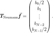
Applying the eigenvalue equation (either apply the new form, or scale the endpoint by a factor of
) we obtain the consistency
condition:
which gives
 , implying that
 . This gives the lattice:
x   x   x   ... x   x
|---|---|-- ... |---|
0   d  2d   ...     L
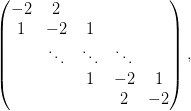
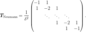
Periodic Boundary Conditions
Periodic boundary conditions are implemented by the operator .. math:
\mat{T}_{\text{Periodic}} = \frac{1}{\delta^2}\begin{pmatrix}
   -2 &  1 \\
    1 & -2 & 1 \\
      & \ddots & \ddots & \ddots \\
      &   &  1 & -2 & 1  \\
    1 &   &    &  1  & -2 \\
  \end{pmatrix}.
This can be represented by the stencil on the augmented
array ![[a,b,\cdots x,y] \rightarrow [y,a,b,\cdots, x,y,a]](../_images/math/93a21a0a7889ff962f6e3cc0f197f977bf619c50.png) . This is
both symmetric and satisfies the charge neutrality condition. Its
structure is preserved by the interpolation and restriction operators:
. This is
both symmetric and satisfies the charge neutrality condition. Its
structure is preserved by the interpolation and restriction operators:
The abscissa and number of lattice points for these are:
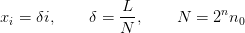
0    x    x    x    x   ... x    x    o
|----|----|----|----|-- ... |----|----|
-d   0    d   2d   3d   ...     L-d   0    = x
-1   0    1    2    3   ...N-2  N-1   0    = N
     R    B    R    B       B    R
Smoothers
Finally, one needs to provide a smoothing operator for this system. The standard choices are weighted Jacobian and some sort of Gauss-Seidel. These are provided by the class MultigridNeumann and MultigridPeriodic which inherit functionality from MultigridBase:
- class mmf.math.multigrid.notes.multigrid_notes.MultigridBase(*varargin, **kwargs)[source]
Common base for MultigridNeumann and MultigridPeriodic.
MultigridBase(n_0=2,
              n=7,
              neutralize=False,
              smoothing_method=0,
              n_smooth=[2,
              2])
Attributes
- class mmf.math.multigrid.notes.multigrid_notes.MultigridNeumann(*varargin, **kwargs)[source]
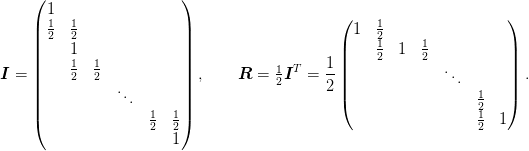
Multigrid class for use with Neumann boundary conditions. The interpolation and restriction operators here are:
MultigridNeumann(n_0=2,
                 n=7,
                 neutralize=False,
                 smoothing_method=0,
                 n_smooth=[2,
                 2],
                 inclusive=False)
which preserve the Galerkin condition for operators of the form
in the sense that
 has the
same tridiagonal form. In addition, the operator satisfies the
symmetry and charge-neutrality conditions:
has the
same tridiagonal form. In addition, the operator satisfies the
symmetry and charge-neutrality conditions:
One has the following sequence of grid sizes:
Attributes
- class mmf.math.multigrid.notes.multigrid_notes.MultigridPeriodic(*varargin, **kwargs)[source]
Multigrid class for use with Periodic boundary conditions. The interpolation and restriction operators here are:
MultigridPeriodic(n_0=2,
                  n=7,
                  neutralize=False,
                  smoothing_method=0,
                  n_smooth=[2,
                  2])
The restriction matrix for
 and
and  is
is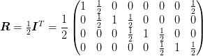
The interpolation matrix for
and  is
is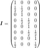
which preserve the Galerkin condition for operators of the form
 (yet to check)
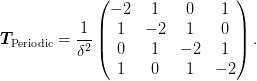
in the sense that
has the
same tridiagonal form. In addition, the operator satisfies the
symmetry and charge-neutrality conditions:One has the following sequence of grid sizes:

Attributes
Demonstration
Here we demonstrate some of the properties of this system. First, we estimate the discretization error. The centered difference formula has an error:

Here we check this for both inclusive and regular grids:
>>> import mmf.math.multigrid.notes.multigrid_notes as MN
>>> import numpy as np
>>> mg = MN.MultigridNeumann(inclusive=False)
>>> x = mg.x()
>>> dx = x[1]-x[0]
>>> y = np.cos(pi*x)
>>> ddy = -np.pi**2*y
>>> d4y = np.pi**4*y
>>> abs((mg.T(y) - ddy) - dx**2*d4y/12).max() < 3*dx**4
True

Remember that we need to divide the endpoints by 2 for inclusive
lattices:
>>> mg = MN.MultigridNeumann(inclusive=True)
>>> x = mg.x()
>>> dx = x[1]-x[0]
>>> y = np.cos(pi*x)
>>> ddy = -np.pi**2*y
>>> ddy[[0,-1]] /= 2
>>> d4y = np.pi**4*y
>>> d4y[[0,-1]] /= 2
>>> abs((mg.T(y) - ddy) - dx**2*d4y/12).max() < 3*dx**4
True
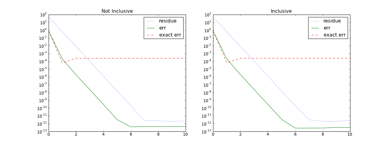
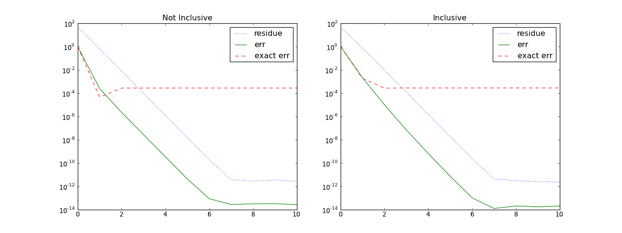
Problem 0 Neumann
Now we check the multigrid convergence for problem version 0.
import mmf.math.multigrid.notes.multigrid_notes as MN
mg = MN.MultigridNeumann(inclusive=False)
x = mg.x(); dx = x[1]-x[0]
f = mg.make_neutral(mg.problem.f(x))
b = mg.problem.b(x)
A = mg.to_mat(mg.A, len(f))
f_ = mg.make_neutral(np.linalg.lstsq(A, b)[0])
g = 0*x
res = [abs(mg.residue(g, b)).max()]
err = [abs(g - f).max()]
err_ = [abs(g - f_).max()]
for n in xrange(10):
   g = mg.make_neutral(mg.f_cycle(g, b))
   res.append(abs(mg.residue(g, b)).max())
   err.append(abs(g - f).max())
   err_.append(abs(g - f_).max())

plt.figure(figsize=(16,6))
plt.subplot(121)
plt.semilogy(res, ':', label='residue')
plt.semilogy(err_, '-', label='err')
plt.semilogy(err, '--', label='exact err')
plt.legend()
plt.title('Not Inclusive')

mg = MN.MultigridNeumann(inclusive=True)
x = mg.x(); dx = x[1]-x[0]
f = mg.make_neutral(mg.problem.f(x))
b = mg.problem.b(x)
A = mg.to_mat(mg.A, len(f))
b[[0,-1]] /= 2                      # Correct the endpoints
f_ = mg.make_neutral(np.linalg.lstsq(A, b)[0])
g = 0*x
res = [abs(mg.residue(g, b)).max()]
err = [abs(g - f).max()]
err_ = [abs(g - f_).max()]
for n in xrange(10):
   g = mg.f_cycle(g, b)
   res.append(abs(mg.residue(g, b)).max())
   err.append(abs(g - f).max())
   err_.append(abs(g - f_).max())

plt.subplot(122)
plt.semilogy(res, ':', label='residue')
plt.semilogy(err_, '-', label='err')
plt.semilogy(err, '--', label='exact err')
plt.legend()
plt.title('Inclusive')
(Source code, png, hires.png, pdf)

Note
The only difference in the multigrid code between inclusive and not inclusive is that the abscissa and volumes are different. We must manually take care of two aspects: Dividing the endpoints of b by 2, and using the proper trapezoidal rule for determining the constant to subtract (which also includes factors of 2 at the endpoints). The latter is done by MultigridNeumann.make_neutral().
Note also that we did not set the attribute MultigridNeumann.neutralize which would have neutralized the solution at each step. It is generally sufficient to do this only at the end of the whole process.
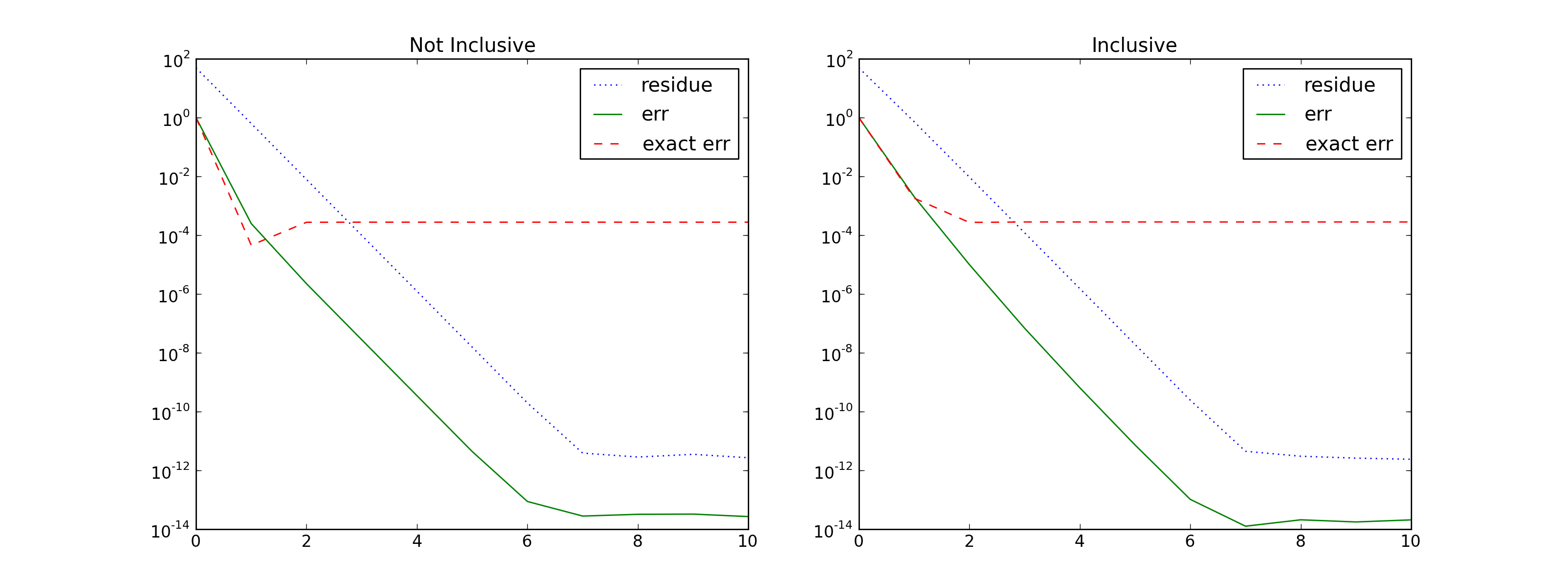
Problem 1 Neumann
Now lets try with the other forms of the problems. Here is the problem version 1.
import mmf.math.multigrid.notes.multigrid_notes as MN
mg = MN.MultigridNeumann(inclusive=False, prob=1)
x = mg.x(); dx = x[1]-x[0]
f = mg.problem.f(x)
b = mg.problem.b(x)
A = mg.to_mat(mg.A, len(f))
f_ = np.linalg.solve(A, b)

g = 0*x
res = [abs(mg.residue(g, b)).max()]
err = [abs(g - f).max()]
err_ = [abs(g - f_).max()]
for n in xrange(10):
   g = mg.f_cycle(g, b)
   res.append(abs(mg.residue(g, b)).max())
   err.append(abs(g - f).max())
   err_.append(abs(g - f_).max())

plt.figure(figsize=(16,6))
plt.subplot(121)
plt.semilogy(res, ':', label='residue')
plt.semilogy(err_, '-', label='err')
plt.semilogy(err, '--', label='exact err')
plt.legend()
plt.title('Not Inclusive')

mg = MN.MultigridNeumann(inclusive=True, prob=1)
x = mg.x(); dx = x[1]-x[0]
f = mg.problem.f(x)
b = mg.problem.b(x)
A = mg.to_mat(mg.A, len(f))
b[[0,-1]] /= 2                      # Correct the endpoints
f_ = np.linalg.solve(A, b)
g = 0*x
res = [abs(mg.residue(g, b)).max()]
err = [abs(g - f).max()]
err_ = [abs(g - f_).max()]
for n in xrange(10):
   g = mg.f_cycle(g, b)
   res.append(abs(mg.residue(g, b)).max())
   err.append(abs(g - f).max())
   err_.append(abs(g - f_).max())

plt.subplot(122)
plt.semilogy(res, ':', label='residue')
plt.semilogy(err_, '-', label='err')
plt.semilogy(err, '--', label='exact err')
plt.legend()
plt.title('Inclusive')
(Source code, png, hires.png, pdf)

Note
For this version of the problem, the matrix is not singular and MultigridNeumann.make_neutral() should not be called.
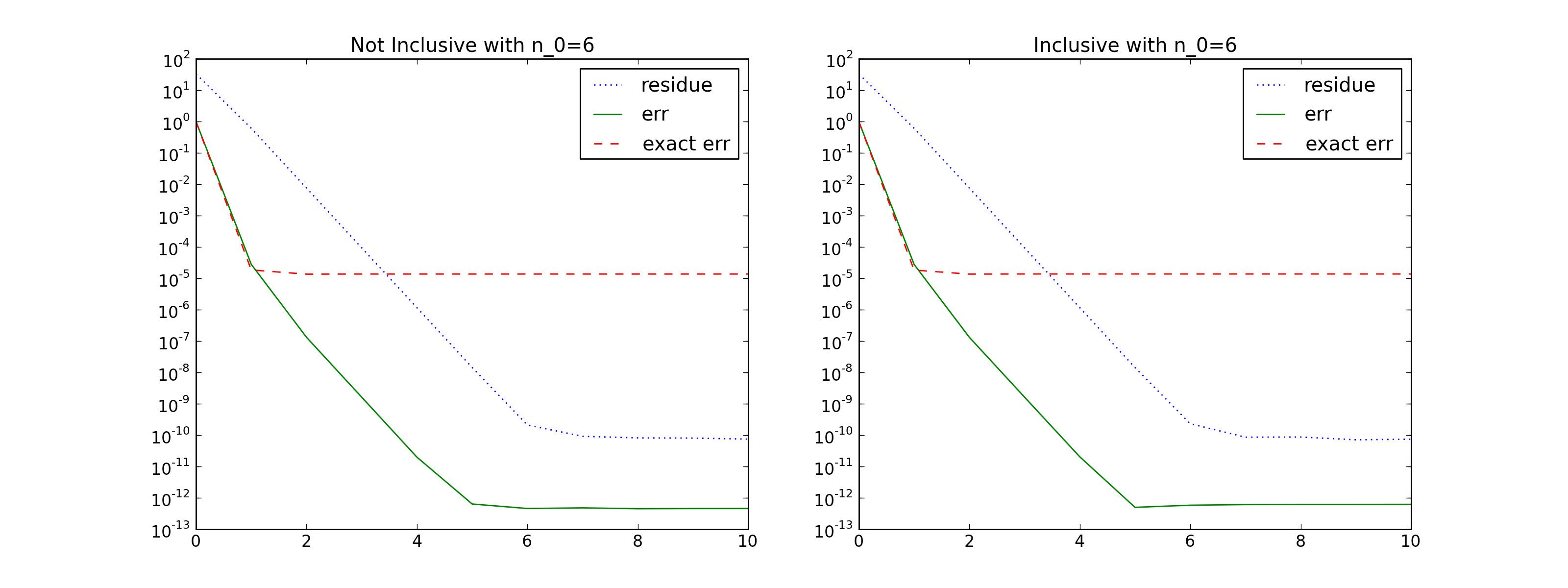
Problem 2 Neumann
And now here is the problem version 2. This case is a bit more
challenging because there are now negative eigenvalues since the
diagonals are no longer positive. However, the spectrum of  which scales as
  still dominates once the lattice is
sufficiently large, so the negative eigenvalues correspond to small
eigenvalues of : i.e. low frequency. Thus, the problem still
has good smoothing properties even though the smoothing is divergent.
still dominates once the lattice is
sufficiently large, so the negative eigenvalues correspond to small
eigenvalues of : i.e. low frequency. Thus, the problem still
has good smoothing properties even though the smoothing is divergent.
The price is that one must terminate the multigrid at a sufficiently
high level and solve the coarse system exactly to remove the
low-frequency errors. in this present case, we find that  works. With
  fixed at
  the method converges as quickly as for
larger values as is shown below:
the method converges as quickly as for
larger values as is shown below:
import mmf.math.multigrid.notes.multigrid_notes as MN
mg = MN.MultigridNeumann(inclusive=False, n_0=6, prob=2)
x = mg.x(); dx = x[1]-x[0]
f = mg.problem.f(x)
b = mg.problem.b(x)
A = mg.to_mat(mg.A, len(f))
f_ = np.linalg.solve(A, b)

g = 0*x
res = [abs(mg.residue(g, b)).max()]
err = [abs(g - f).max()]
err_ = [abs(g - f_).max()]
for n in xrange(10):
   g = mg.f_cycle(g, b)
   res.append(abs(mg.residue(g, b)).max())
   err.append(abs(g - f).max())
   err_.append(abs(g - f_).max())

plt.figure(figsize=(16,6))
plt.subplot(121)
plt.semilogy(res, ':', label='residue')
plt.semilogy(err_, '-', label='err')
plt.semilogy(err, '--', label='exact err')
plt.legend()
plt.title('Not Inclusive with n_0=%i' % (mg.n_0))

mg = MN.MultigridNeumann(inclusive=True, n_0=6, prob=2)
x = mg.x(); dx = x[1]-x[0]
f = mg.problem.f(x)
b = mg.problem.b(x)
A = mg.to_mat(mg.A, len(f))
b[[0,-1]] /= 2                      # Correct the endpoints
f_ = np.linalg.solve(A, b)
g = 0*x
res = [abs(mg.residue(g, b)).max()]
err = [abs(g - f).max()]
err_ = [abs(g - f_).max()]
for n in xrange(10):
   g = mg.f_cycle(g, b)
   res.append(abs(mg.residue(g, b)).max())
   err.append(abs(g - f).max())
   err_.append(abs(g - f_).max())

plt.subplot(122)
plt.semilogy(res, ':', label='residue')
plt.semilogy(err_, '-', label='err')
plt.semilogy(err, '--', label='exact err')
plt.legend()
plt.title('Inclusive with n_0=%i' % (mg.n_0))
(Source code, png, hires.png, pdf)
Note
For this version of the problem, the matrix is not singular and MultigridNeumann.make_neutral() should not be called.
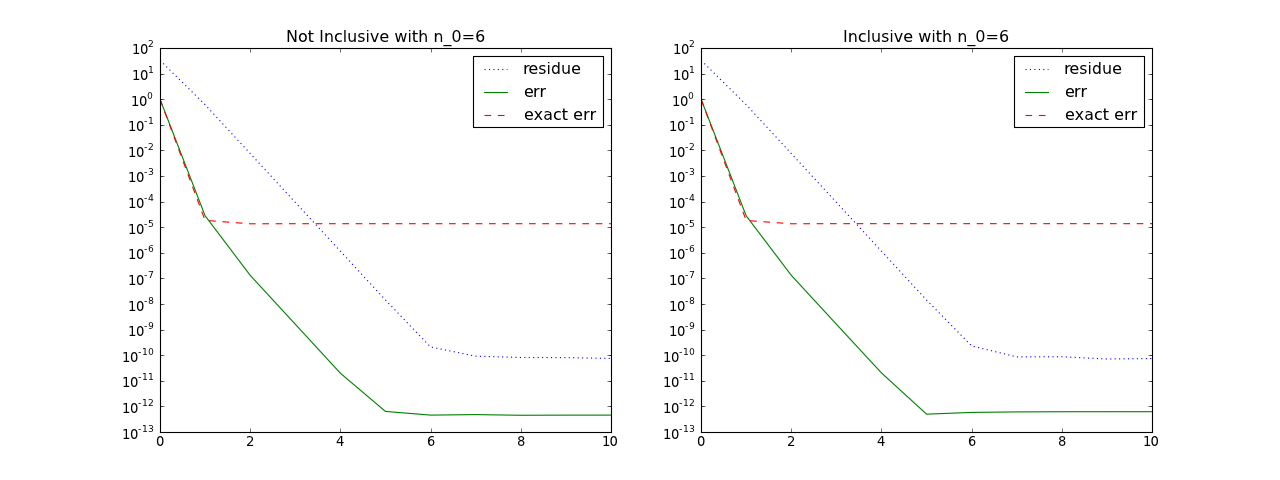
Newtons Method Neumann
Now we try the Newton iteration as a method for solving the non-linear equations. First we start with the solution and check that the Newton equation can be solver with the multigrid algorithm. We first start with a smooth deviation from the solution: .. plot:
:width: 100%
:include-source:

import mmf.math.multigrid.notes.multigrid_notes as MN
mg = MN.MultigridNeumann(inclusive=False, n_0=6, prob=3)
x = mg.x(); dx = x[1]-x[0]
f = mg.problem.f(x)
g = mg.problem.g(x)

df = 0*f + 0.01                # Constant shift to make like easy
dg = 0*g + 0.01
fg = np.vstack((f, g))
dfg = np.vstack((df, dg))

dG = mg.problem.DJ(dfg=dfg, f=f, g=g, x=x)
b = -mg.T()mg.problem.DG(fg=fg, x=x)
A = mg.to_mat(mg.A, len(f))
f_ = np.linalg.solve(A, b)

g = 0*x
res = [abs(mg.residue(g, b)).max()]
err = [abs(g - f).max()]
err_ = [abs(g - f_).max()]
for n in xrange(10):
   g = mg.f_cycle(g, b)
   res.append(abs(mg.residue(g, b)).max())
   err.append(abs(g - f).max())
   err_.append(abs(g - f_).max())

plt.figure(figsize=(16,6))
plt.subplot(121)
plt.semilogy(res, ':', label='residue')
plt.semilogy(err_, '-', label='err')
plt.semilogy(err, '--', label='exact err')
plt.legend()
plt.title('Not Inclusive with n_0=%i' % (mg.n_0))

mg = MN.MultigridNeumann(inclusive=True, n_0=6, prob=2)
x = mg.x(); dx = x[1]-x[0]
f = mg.problem.f(x)
b = mg.problem.b(x)
A = mg.to_mat(mg.A, len(f))
b[[0,-1]] /= 2                      # Correct the endpoints
f_ = np.linalg.solve(A, b)
g = 0*x
res = [abs(mg.residue(g, b)).max()]
err = [abs(g - f).max()]
err_ = [abs(g - f_).max()]
for n in xrange(10):
   g = mg.f_cycle(g, b)
   res.append(abs(mg.residue(g, b)).max())
   err.append(abs(g - f).max())
   err_.append(abs(g - f_).max())

plt.subplot(122)
plt.semilogy(res, ':', label='residue')
plt.semilogy(err_, '-', label='err')
plt.semilogy(err, '--', label='exact err')
plt.legend()
plt.title('Inclusive with n_0=%i' % (mg.n_0))