Solving Nonlinear Equations¶

We use the test problems defined in mmf.solve.test_problems.

Minimization versus Root Finding¶

Minimization problems have the advantage that one can always determine the downhill direction from the gradient, thus one can ensure that an iteration will improve and succeed (unless there are pathologies).

However, from a local sense, convergence is difficult because one needs to find the minimum of a “flat” function (typically quadratic at the solution). It is much more efficiently locally to find the root of the derivatives as the function is typically linear here and Newton or Quasi-Newton methods work very well here once the solution is isolated. However, ensuring global convergence is difficult. The ideal situation is to use both, applying the minimization principle to guarantee convergence while using the stationary conditions to polish the root.

In general, one may need to solve a set of equations that do not correspond to a minimization problem. Thus, we are simply presented with a set of equations to solve

$\vect{G}(\vect{x}) = 0.$

One can visualize this as a minimization problem $F = \norm{\vect{G}}^2$ , however, this will typically introduce many spurious local minima and it should therefore not be treated as a minimization problem. However, is useful to consider the gradient of this function, as this is related to the Jacobian $\mat{J}_{ij} = \nabla_{j}G_{i}$ of Newton’s method:

$\vect{\nabla}{F} = 2\vect{G}\nabla\vect{G} = 2\vect{G}^{\dagger}\cdot\mat{J}.$

This is useful in quasi-Newton methods to ensure termination. In particular, given a step $\lambda\d{\vect{x}}$ , the change in the objective function should approach

$\d{F} = \lambda\vect{\nabla}{F}\cdot\d{\vect{x}} \approx 2\lambda \vect{G}^{\dagger}\cdot\mat{J}\cdot\d{\vect{x}} = 2\lambda F$

where the last relationship is valued due to the secant constraint $\d{\vect{G}} = \mat{J}\d{\vect{x}}$ with $\mat{J}$ being the approximation to the Jacobian.

Examples¶

Mexican Hat¶

As a first example, we consider minimization of a Mexican hat potential mmf.solve.test_problems.TwoDimensional.MexicanHat. Here is the potential we are minimizing $f(x,y)$ as well as the root-finding potential $F(x,y) = f_{,x}^2 + f_{,y}^2$ :

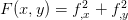from mmf.solve.test_problems import TwoDimensional

from mpl_toolkits.mplot3d import Axes3D
from matplotlib import cm

potential = TwoDimensional.MexicanHat()
r = np.linspace(0,1.3,40)
theta = np.linspace(0,2*np.pi,40)
R, Theta = np.meshgrid(r, theta)
X = R*np.cos(Theta)
Y = R*np.sin(Theta) + 1.0
Z = potential.f(X, Y)

fig = plt.figure(figsize=[16,6])
ax = Axes3D(fig, [0,0,0.5,1])
ax.plot_surface(X, Y, Z, rstride=1, cstride=1, color='b')

r = np.linspace(0,1.1,40)
theta = np.linspace(0,2*np.pi,40)
R, Theta = np.meshgrid(r, theta)
X = R*np.cos(Theta)
Y = R*np.sin(Theta) + 1.0
Z = potential.F(X, Y)

ax = Axes3D(fig, [0.5,0,0.5,1])
ax.plot_surface(X, Y, Z, rstride=1, cstride=1, color='r')
ax.azim = -23
ax.elev = 65
plt.draw()

(Source code, png, hires.png, pdf)

We can see that the function $F(x)$ has much more pronounced features – making it easier to solve locally – but also has many more minima because all stationary points satisfy the equations of motion. Thus, there is a chance that one might fall into the wrong solution.

Now we consider:

from mmf.solve.test_problems import TwoDimensional

potential = TwoDimensional.MexicanHat()

def f(x):
    x0 = x - 1
    while np.linalg.norm(x - x0) > 0.00001:
       x0 = x
       x = x - np.dot(potential.Jinv(x[0], x[1]),
                      potential.G(x))
    return x

extent = [-1,1,0,2.5]
x = np.linspace(extent[0], extent[1], 400)
y = np.linspace(extent[2], extent[3], 400)
C = zeros((len(x), len(y)), dtype=int)
r = [np.array([0, 0]),
     np.array([0, (3 + np.sqrt(1 - potential.b))/2]),
     np.array([0, (3 + np.sqrt(1 + potential.b))/2])]
for nx, x_ in enumerate(x):
    print x_
    for ny, y_ in enumerate(y):
        c = f(array([x_, y_]))
        if np.linalg.norm(c - r[0]) <= 0.01:
            C[nx, ny] = 1
        elif np.linalg.norm(c - r[1]) <= 0.01:
            C[nx, ny] = 2
        elif np.linalg.norm(c - r[2]) <= 0.01:
            C[nx, ny] = 3
        else:
            C[nx, ny] = 0

plt.imshow(np.flipud(C.T), extent=extent)

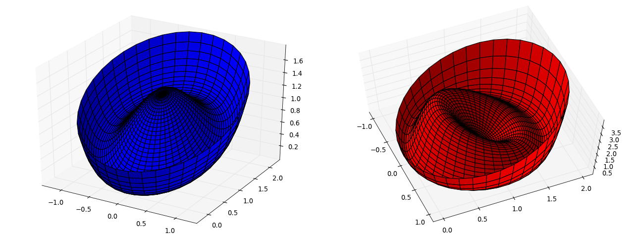
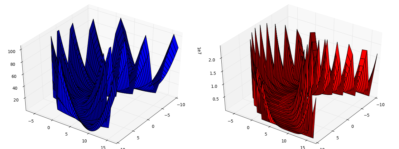
Sensitive Parameters¶

Here we consider the minimization of a different potential with a “sensitive parameter”: mmf.solve.test_problems.TwoDimensional.SensitiveParameter.

This consists of a smooth parabolic valley with nasty fluctuations away from the valley. The potential is constructed in such a way so that the function f(x,y) is a parabola when x is held fixed, thus, a good strategy is to hold x fixed, minimize for y and then consider changing x.

from mmf.solve.test_problems import TwoDimensional

from mpl_toolkits.mplot3d import Axes3D
from matplotlib import cm

potential = TwoDimensional.SensitiveParameter()
x = np.linspace(-10,10,40)
y = np.linspace(-7,7,40)
X, Y = np.meshgrid(x, y)
Y = Y + potential.c*X**2
Z = potential.f(X, Y)

fig = plt.figure(figsize=[16,6])
ax = Axes3D(fig, [0,0,0.5,1])
ax.plot_surface(X, Y, Z, rstride=1, cstride=1, color='b')
ax.azim = 35.0625
ax.elev = 39.75

Z = potential.F(X, Y)
ax = Axes3D(fig, [0.5,0,0.5,1])
ax.plot_surface(X, Y, Z, rstride=1, cstride=1, color='r')
ax.azim = 35.0625
ax.elev = 39.75
plt.draw()

(Source code, png, hires.png, pdf)

Here we show the trajectories.

from mmf.solve.test_problems import TwoDimensional
from mmf.solve.solver_interface import solve, IterationError
from mmf.solve.broyden_solvers import Broyden

potential = TwoDimensional.SensitiveParameter()
solver = Broyden(verbosity=0, debug=True)

#make contour plot
x = np.linspace(-1,12,1000)
y = np.linspace(-13,15,1000)
X, Y = np.meshgrid(x, y)
Z = potential.f(X, Y)
axis = [-1,12,-13,15]

plt.contour(X,Y,Z**(0.1), 10, zorder=-1000)

# First attempt: Solve along good orthogonal directions.
def f(x):
    def g(y):
        xs.append(x)         # Keep track of path.
        ys.append(y)
        return potential.f_y(x,y)
    y0[0] = solve(f=g, x0=y0[0], solver=solver).x_[0]
    y_ = np.array(zip(*solver._debug.steps)[0])
    ys_.extend(y_)
    xs_.extend(0*y_ + x)

    return potential.f(x, y0[0])

y0 = [9]
xs, ys = [], []              # All points sampled
xs_, ys_ = [], []            # Points actually tried

solve(f=f, x0=9, solver=solver).x_[0];

xs, ys, xs_, ys_ = map(lambda x: np.asarray(x).ravel(),
                       [xs, ys, xs_, ys_])
plt.plot(xs, ys, 'b.',zorder=101)
plt.plot(xs_, ys_, 'b-x',zorder=101)
dx = np.diff(xs_)
dy = np.diff(ys_)
for n in xrange(len(dx)):
    a = plt.arrow(xs_[n], ys_[n], dx[n]/2, dy[n]/2,
                  linewidth=0, head_width=0.2, zorder=100,
                  color='b')

# Now try full solving: this fails!
def F(x):
    xs.append(x[0]); ys.append(x[1])
    return np.array([potential.f_x(x[0], x[1]), potential.f_y(x[0], x[1])])

xs, ys = [], []
try:
    solve(f=F, x0=[9,9], solver=solver)
except IterationError:
    pass


plt.plot(xs, ys, 'rx', zorder=200)
xys = np.array(zip(*solver._debug.steps)[0])


plt.plot(xys[:,0], xys[:,1], 'x-r',zorder=200)
dx = np.diff(xys[:,0])
dy = np.diff(xys[:,1])
for n in xrange(len(dx)):
    a = plt.arrow(xys[n,0], xys[n,1], dx[n]/2, dy[n]/2,
                  linewidth=0, head_width=0.01, zorder=200,
                  color='r')

# Even Newton's method has difficulty:
xs, ys = [], []
x = y = 9
for n in xrange(100):
    xs.append(x); ys.append(y)
    x, y = np.array([x,y]) - np.dot(potential.Jinv(x, y), F([x,y]))

plt.plot(xs, ys, 'g:x',zorder=99)
dx = np.diff(xs)
dy = np.diff(ys)
for n in xrange(len(dx)):
    a = plt.arrow(xs[n], ys[n], dx[n]/2, dy[n]/2,
                  linewidth=0, head_width=0.2, zorder=99,
                  color='g')

plt.axis(axis)

(Source code, png, hires.png, pdf)

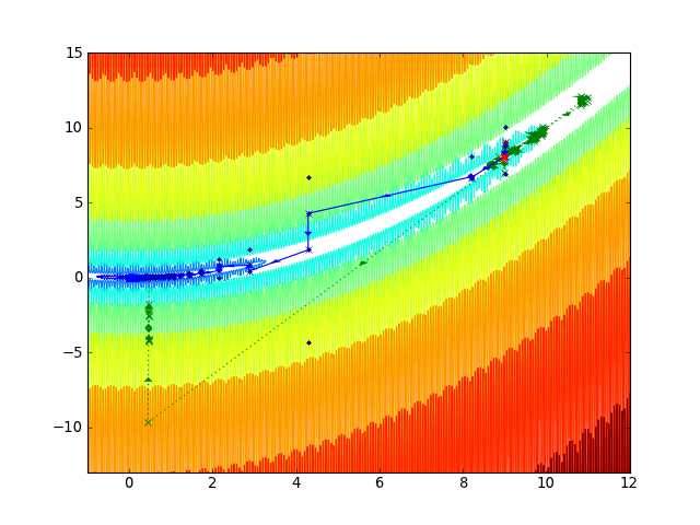
First we hold the sensitive parameter x fixed and solve for g(y): this always succeeds rapidly as the function is quadratic. Then we treat this as a new function of f(x) and solve for it, which walks down the valley (blue line). Then we try to apply a Broyden solver to the full function (green line). This fails miserably. (Note, because of the quadratic form, Newton’s method (green) actually works, although slowly, because each step takes it right down into the valley. A more typical example would not have this property.

Table Of Contents

Previous topic

Next topic

This Page

Solving Nonlinear Equations¶

Minimization versus Root Finding¶

Examples¶

Mexican Hat¶

Sensitive Parameters¶

Navigation

Table Of Contents

Previous topic

Next topic

This Page

Quick search

Solving Nonlinear Equations¶

Minimization versus Root Finding¶

Examples¶

Mexican Hat¶

Sensitive Parameters¶

Navigation