Multigrid Method
Here we present some notes about the multigrid method.
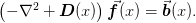
The mmf.math.multigrid module provides efficient ways of solving Poisson-type equations:
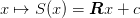
The geometric version of the problem presents a discretization of the left-hand side on a sequence of finer grids.
Details
Here we implements some simple multigrid solvers. These solve a series of related linear problems

where the matrices  have special properties, typically
representing derivative operators such as the Laplacian on a
series of grids of increasing size.
have special properties, typically
representing derivative operators such as the Laplacian on a
series of grids of increasing size.
Formally, the problem requires a set of three operators:
: A restriction operator that
- takes a right hand side of the problem on a finer grid into a right-hand side on a coarser grid.
: A smoothing operator that removes
- high-frequency components of the error from the solution.
: An interpolation operator that
- takes a solution on a coarser grid into a solution on the finer grid.
Typically these are linear operators (and we shall consider only linear operators here) and should satisfy the Galerkin condition:

which serves to define the coarse grid operators  in terms of
the finer grid operator. A second condition is usually imposed that
the interpolation and restriction operations be related by transposition:
in terms of
the finer grid operator. A second condition is usually imposed that
the interpolation and restriction operations be related by transposition:

This helps with the analysis by defining a variational property:
Note
I think this states that the solution to the coarse problem provides the
minimum error solution to the fine problem when interpolated. In other
words, if we only consider solutions of the form  , then the best solution (in the sense of minimizing the
error
, then the best solution (in the sense of minimizing the
error  ) in this subspace will be the
interpolation of the solution
) in this subspace will be the
interpolation of the solution  to the coarsened problem.
However, I can’t prove this right now.
to the coarsened problem.
However, I can’t prove this right now.
As we shall see, the Galerkin condition is not always easily maintained if efficient matrix operation is desired.
The smoothing operator  must provide a relaxation method for
the problem. The efficiency of the multigrid method is based on each
of these operations being able to be applied in
must provide a relaxation method for
the problem. The efficiency of the multigrid method is based on each
of these operations being able to be applied in  time where
 is the number of unknowns. These are typically just weighted
averages of nearest neighbours respecting this requirement.
is the number of unknowns. These are typically just weighted
averages of nearest neighbours respecting this requirement.
The idea is for one to use  to damp the high frequency errors, then
to recursively apply the algorithm using
to damp the high frequency errors, then
to recursively apply the algorithm using  and
and  to go to a
coarser grid. In the coarser grid, the low-frequency errors become
high frequency errors which are again damped. Typically, this is
accomplished with a weighted Jacobi algorithm or red-black ordered
Gauss-Seidel. The idea is to form an update
to go to a
coarser grid. In the coarser grid, the low-frequency errors become
high frequency errors which are again damped. Typically, this is
accomplished with a weighted Jacobi algorithm or red-black ordered
Gauss-Seidel. The idea is to form an update
that is idempotent on the solution  . This ensures that the
errors grow as
. This ensures that the
errors grow as  .
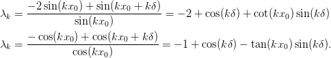
This, then eigenvalues of
.
This, then eigenvalues of  control the convergence: thus one
chooses the iteration in such a way that the eigenvalues of
high-frequency components are substantially between 1 and -1. The
choice of is discussed in detail in the section
Smoothing below.
control the convergence: thus one
chooses the iteration in such a way that the eigenvalues of
high-frequency components are substantially between 1 and -1. The
choice of is discussed in detail in the section
Smoothing below.
Discretization
The first step, however, is to consider the discretization of the
Poisson operator  . This should have several
properties:
. This should have several
properties:
As the Laplacian is a symmetric operator (in the sense that all the eigenvalues are real), the discretization should preserve this property. This requires a fairly careful implementation of the boundary conditions.
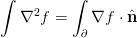
The Laplacian should preserve charge neutrality with applicable boundary conditions: the finite version of integration-by-parts:
Thus, with Neumann boundary conditions or without a boundary (for example, if one has periodic boundary conditions), for any vector
 one should have
  which means
 . (For Dirichlet boundary conditions, one
must include the boundary contribution and so this relationship
will not hold at the boundaries).
. (For Dirichlet boundary conditions, one
must include the boundary contribution and so this relationship
will not hold at the boundaries).In addition, the equation
 will have a
solution iff
will have a
solution iff  . This means that
  must have a
singular direction. This must be considered when solving such
systems.
must have a
singular direction. This must be considered when solving such
systems.
The second question is the order of the discretization. Apparently, for the multigrid method, higher order is not very helpful, so we content ourselves with the symmetric differences scheme.
We consider the following operators for the second derivatives which
satisfy these properties. Each of these can be expressed as
 in
terms of forward and backward difference operators:
in
terms of forward and backward difference operators:
We must, however, determine the consistent abscissa. This is done by
consider the plane-wave wavefunctions  . For intermediate
points with spacing
. For intermediate
points with spacing  we immediately find the eigenvalues

We now consider the endpoints. Let the left endpoint be at  ,
we then have the following condition obtained at the left endpoint
with
,
we then have the following condition obtained at the left endpoint
with  for Dirichlet and
  for Neumann boundary
conditions respectively (the periodic condition place no restrictions):
for Neumann boundary
conditions respectively (the periodic condition place no restrictions):
A consistent discretization will have a solution for all  which
leads to the following consistency conditions:
which
leads to the following consistency conditions:
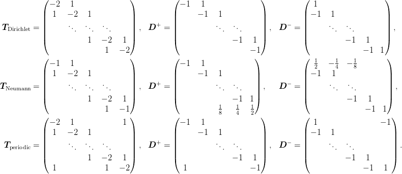
Dirichlet
Here we have  , which is always satisfied
if
, which is always satisfied
if  :
:
o    x    x    x   ...   x    o
|----|----|----|-- ... --|----|
0   1d   2d   2d   ...  Nd    L
Hence, given the interval ![[0,L]](../_images/math/075f61eea4c937b38e3d94399c58bbd9d7281bce.png) with the
Dirichlet conditions
with the
Dirichlet conditions  , the discretization is valid for
the lattice points
, the discretization is valid for
the lattice points
Neumann
Here we have  , which is always
satisfied if
, which is always
satisfied if  :
:
o  x    x    x   ... x    x  o
|--|----|----|-- ... |----|--|
0 d/2 3d/2 5d/2  ...         L
Here is a little check of the Neumann case. We first form the eigenvectors and eigenvalues, and then show that we recover the desired form of operator:
>>> L = 1
>>> N = 4
>>> f = 0.5
>>> d = L/(N - 1 + 2*f)
>>> x0 = f*d
>>> x = np.ogrid[x0:L-x0:N*1j]
>>> n = np.arange(N)
>>> k = pi*n/L
>>> V = np.cos(k[None,:]*x[:,None])
>>> V = 1/np.sqrt(np.diag(np.dot(V.T, V)))*V
>>> E = 2*(cos(k*d) - 1).ravel()
>>> T = np.dot(np.dot(V, diag(E)), V.T).round(2)
>>> T
array([[-1.,  1., -0.,  0.],
       [ 1., -2.,  1., -0.],
       [-0.,  1., -2.,  1.],
       [ 0., -0.,  1., -1.]])
One difficulty with the Neumann boundary conditions is that they don’t
lend themselves to trivial restriction and interpolation: There is no
way of removing lattice sites while preserving the ratio  . One has several options:
Choose a different parametrization of
that lends itself
to simple restriction and interpolation. One way to do this is to
include the endpoint as part of the grid (i.e.  ). The
discretization is then
). The
discretization is then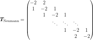
Unfortunately this fails both the symmetry and neutrality criteria.
Keep the current form of diagonalization but choose a modified restriction and interpolation to preserve the grid properties. The complication here is that the lattice points of the coarser grid will not coincide with those of finer grids.
Keep the current form of diagonalization and the trivial restriction and interpolation and hope that the method will work. This may still work if we impose the Galerkin principle. Let’s try this in one dimension on the following problem:
These may be considered as a test problem with periodic boundary conditions on
![[0,2]](../_images/math/9076ffb2b9c051f1b6f07bf18066581d57216258.png) or with Neumann boundary conditions on
or with Neumann boundary conditions on
![[0,1]](../_images/math/e861e10e1c19918756b9c8b7717684593c63aeb8.png) . We use the following refinement with
. We use the following refinement with  grid-points:
|        x               x       |       n0     = 2
    |    x       x       x   |         1 n0 + 1 = 3
       | x   x   x   x   x |           2 n0 + 1 = 5
        |x x x x x x x x x|            4 n0 + 1 = 9
        0-----------------L
Note that the length of the grid varies from level to level: our hope is that enforcing the Galerkin principle will suffice to ensure good convergence behaviour. The nai{}ve interpolation and restriction operators preserve the form of
 and so
will work with the first form of the problem.
and so
will work with the first form of the problem.
These are probably not very good in that they do not preserve constants at the boundaries, but maybe the Galerkin principle will come to the rescue. We shall take the following problem as an e
Skewed Metric
Another complication arises with a non-trivial metric which we allow
for the purpose of allowing distorted lattices. We allow the user to
provide a matrix  who’s columns are the lattice vectors.
This gives rise to
who’s columns are the lattice vectors.
This gives rise to  , the matrix of displacements
(roughly,
, the matrix of displacements
(roughly,  where
where  is the number of
segments. One must take care to include
is the number of
segments. One must take care to include  appropriately.)
Consider a 2d grid with basis vectors  and
and  :
:

Let  be the operator
 ![[D]_{ij} = \nabla_{i}\nabla_{j}f](../_images/math/0715d863ae42a6f56df7c70e3ecf70ad4a77c960.png) about the point of interest so that
about the point of interest so that

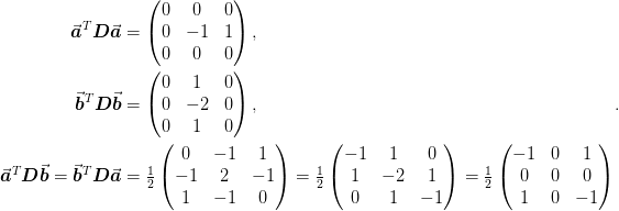
We have the following relationships valid to order  (where we have used the fact that
  :
:
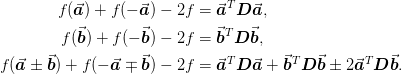
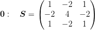
We can compute the Laplacian as follows:
![\nabla^2 = \tr[\mat{D}] = \tr\left[
[\mat{\delta}^{-1}]^T\begin{pmatrix}
\vect{a}^T\mat{D}\vect{a} & \vect{a}^T\mat{D}\vect{b}\\
\vect{b}^T\mat{D}\vect{a} & \vect{b}^T\mat{D}\vect{b}
\end{pmatrix}
\mat{\delta}^{-1}
\right].](../_images/math/3b234bb2a89b40d6b0621baf02423f2b711ebf62.png)
Since the Laplacian is symmetric, 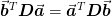 . Furthermore, the multidimensional
matrices may be constructed from the lower dimensional versions using
the tensor product. Thus, we really only need a one dimensional
stencil for
. Furthermore, the multidimensional
matrices may be constructed from the lower dimensional versions using
the tensor product. Thus, we really only need a one dimensional
stencil for  and a two
dimensional stencil for
and a two
dimensional stencil for  .
.
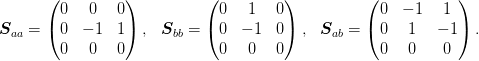
To be explicit, we compute all the two-dimensional stencils.
Let us reshape the operator ![[T]_{x_a, y_a; x_b,y_b}](../_images/math/c3bd0e8e0f533df12b84111e226d750392e6dd45.png) over the
coordinates. It is customary to consider the following 9-point
stencil representing the averaging of the surrounding cells about the
point
over the
coordinates. It is customary to consider the following 9-point
stencil representing the averaging of the surrounding cells about the
point  :
:
![\mat{S}^{a,b} = [T]_{a,b;[a-1:a+1],[b-1:b+1]} =
\begin{pmatrix}
NW & N & NE\\
W & C & E\\
SW & S & SE
\end{pmatrix}
=
\begin{pmatrix}
S^{a,b}_{-,-} & S^{a,b}_{-,0} & S^{a,b}_{-,+}\\
S^{a,b}_{0,-} & S^{a,b}_{0,0} & S^{a,b}_{0,+}\\
S^{a,b}_{+,-} & S^{a,b}_{+,0} & SS^{a,b}_{+,+}
\end{pmatrix}.](../_images/math/ffe4ffadba063d30b6b7b5b3ce08024c5cc4226b.png)
Denote the indices  , then the symmetry and
neutrality constraints have the form:
, then the symmetry and
neutrality constraints have the form:
For example, in the interior, we have a single stencil  for all
  , thus the conditions reduce to
  and
and  . The
constructions are linear, so we construct a “basis” of
stencils representing the various combinations
. The
constructions are linear, so we construct a “basis” of
stencils representing the various combinations
 that satisfy these properties. Then the
linear combinations required to compute
that satisfy these properties. Then the
linear combinations required to compute  will by
construction also satisfy the properties. In the interior we have the
stencils :
will by
construction also satisfy the properties. In the interior we have the
stencils :

We note that, to order  , there is also a “zero” stencil:
For the Neumann boundary conditions we have the following set of stencils (plus rotations) at the edges:

and at the corner we have:
Now we consider the boundary conditions  . The most
difficult are the lattice Neumann where we have at the point
. The most
difficult are the lattice Neumann where we have at the point
 (see the discussion above about the 1d discretization) that
 . This gives us the additional
relationship
. This gives us the additional
relationship  and so we have:
From this we can from the coordinate transformation :
![\mat{R} = \mat{\delta}^{-1}\cdot[\mat{\delta}^{-1}]^{T}](../_images/math/8575de98eb4ef9451f642458f94445d7eb4404eb.png)
The Laplacian is then
where the matrices are broadcast appropriately such that the summation is over the coordinate axes. This will preserved
Note
The Neumann boundary conditions will not be strictly preserved by this: the derivative will not vanish along the normal to the boundary – which is the usual condition – but will instead vanish along the lattice. This is actually what we want because we are use the Neumann cell to model an octant of the full unit cell in a periodic system.
Smoothing
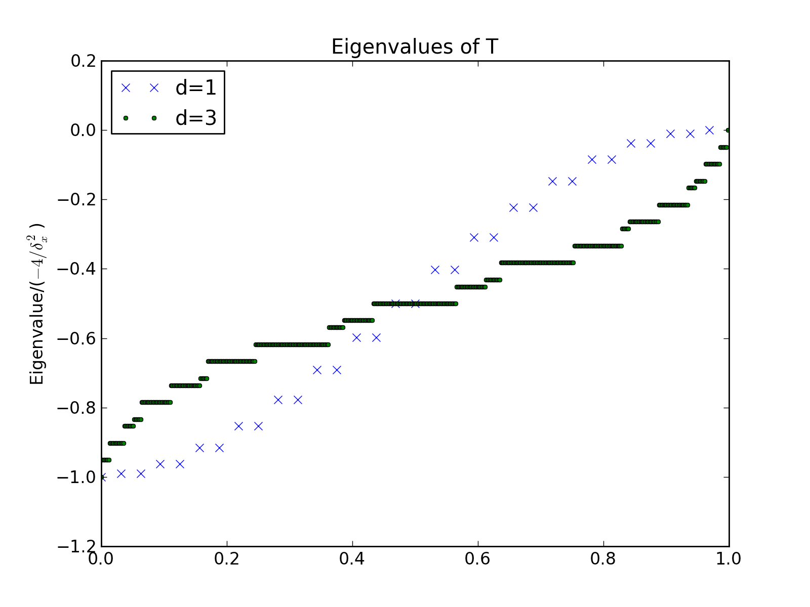
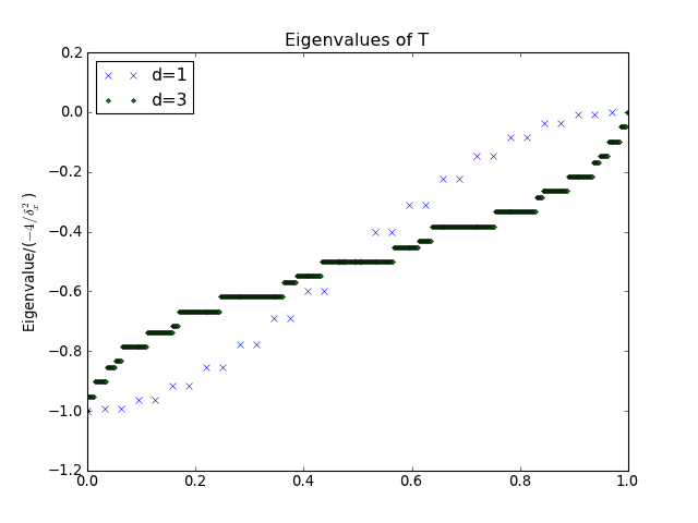
We first consider the form:

Generally  has eigenvalues
Note
The arbitrary metric and dimensionality is incorporated into
the factor  . To see this, consider that the trace sums
over the dimensions of the Laplacian, with each dimension
contributing
. To see this, consider that the trace sums
over the dimensions of the Laplacian, with each dimension
contributing  .
.
import mmf.math.multigrid
mg = mmf.math.multigrid.MG(
    d=1, n_0=1, n=5, L=0.1, boundary_conditions='periodic')
T = -mg.get_mats()[0][-1].toarray()
#T = -mg.to_mat(mg.x()[0], mg.T)
assert np.allclose(T,T.T)
E = np.linalg.eigvalsh(T)
dx_inv2 = np.trace(np.dot(mg.dx_inv().T,mg.dx_inv()))
plt.plot(np.arange(len(E),dtype=float)/len(E),
         E/(4*dx_inv2),
         'x',
         label="d=%i" % (mg.d,))

mg.initialize(n=3, d=3, n_0=(1,1,1))
T = -mg.get_mats()[0][-1].toarray()
#T = -mg.to_mat(mg.x()[0], mg.T)
assert np.allclose(T,T.T)
E = np.linalg.eigvalsh(T)
dx_inv2 = np.trace(np.dot(mg.dx_inv().T,mg.dx_inv()))
plt.plot(np.arange(len(E),dtype=float)/len(E),
         E/(4*dx_inv2),
         '.',
         label="d=%i" % (mg.d,))

plt.legend(loc='upper left')
plt.title("Eigenvalues of T")
plt.ylabel("Eigenvalue/($-4/\delta_x^2$)")
(Source code, png, hires.png, pdf)
In order to ensure idempotency, we want smoothing operation in the form of
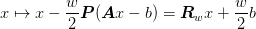
where 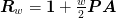 . This
trivially satisfies the idempotency requirement. The goal is to
choose the weight and the matrix
. This
trivially satisfies the idempotency requirement. The goal is to
choose the weight and the matrix  (pre-conditioner) that is
easy to compute (in terms of being of order cost to compute
(pre-conditioner) that is
easy to compute (in terms of being of order cost to compute
 ) such that the eigenvalues of the
  corresponding to high frequency components have magnitude less than
one. In the case of only a constant mass term
corresponding to high frequency components have magnitude less than
one. In the case of only a constant mass term  we may neglect
to obtain
we may neglect
to obtain
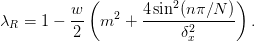
Since our “multigrid” involves coarsening the grid by a factor of two, we wish to minimize the magnitude over the upper half of the frequencies, defining a fitness:
![\mu \approx \max_{\theta\in[\pi/2, \pi]} \abs{\lambda_R}
= \max_{\theta\in[\pi/2, \pi]} \Abs{1 - \frac{w}{2}\left(m^2
+ \frac{4\sin^2(\theta)}{\delta_x^2}\right)}.](../_images/math/d18f670f60dbaa14fd1d26d44eeaa463693a2e64.png)
The extrema occur at the endpoints, and a little inspection tells us that the optimal weight must satisfy:
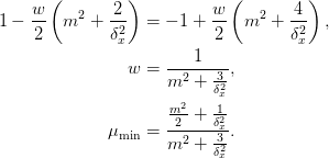
For reasonable problems, in the limit of large lattices, the
 terms dominate, and this approaches
  .
.
This suggests that as a general pre-conditioner we might use:

with a weight of  . The more standard pre-conditioner would be

with as this corresponds directly to the diagonal of  but it is not clear to me yet why this is better.
Finally, recall that we also consider the case where has an
additional matrix structure so it is block diagonal in position space
(rather than strictly diagonal). Here one has the choice of
extracting the diagonal, or spending the extra work to diagonalize
each of the blocks.