mmf.math.multigrid
| notes | |
| stencil | Stencil Module (mmf.math.multigrid.stencil) |
| MG(*varargin, **kwargs) | Multigrid Poisson-like solver. |
| MultiGrid | Multigrid Poisson-like solver. |
| DivergenceError | Raised if the f_cycle fails to reduce the residual, signaling |
| WignerSeitz(*varargin, **kwargs) | This class sets up the spherical Wigner-Seitz approximation to problems of the form |
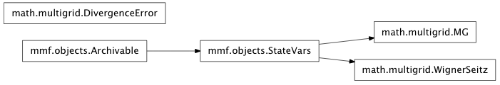
Inheritance diagram for mmf.math.multigrid:
Multigrid Solvers.
This module provides efficient ways of solving Poisson-type equations:

For details, please see the notes in section Multigrid Method.
Todo
Remove parity and fix Neumann boundary conditions!
Todo
Add regression test for bug fixed in version 2553.
- class mmf.math.multigrid.MG(*varargin, **kwargs)
Bases: mmf.objects.StateVars
Multigrid Poisson-like solver.
MG(n=3,
   n_0=2,
   n_min=1024,
   d=3,
   L=None,
   n_smooth=(2,
   2),
   abs_tol=1e-08,
   rel_tol=1e-08,
   boundary_conditions=Neumann,
   periodic_center=True,
   verbosity=0,
   smoothing_algorithm=GSLEX,
   smoothing_weight=1,
   preconditioner=gerschgorin,
   sparse_solver=bicgstab,
   sparse_solver_iterations=0,
   current_state_dir=,
   try_linsolve=True)
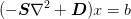
This class solvers problems of the form
The present formulation restricts the boundary conditions to those such that the operator
 can be implemented with a single
stencil acting on an augmented array where the augmented array
contains the neighbouring points. Presently these must be points
within the same grid. This allows one to implement periodic and
Neumann boundary conditions.
can be implemented with a single
stencil acting on an augmented array where the augmented array
contains the neighbouring points. Presently these must be points
within the same grid. This allows one to implement periodic and
Neumann boundary conditions.Notes
Most functions work with a representation x of some function evaluated on the grid or one of the sub-grids. The code allows for a vector-valued function, so one must have x.shape = (n,) + (N,)*d where n is the number of components of the vector-valued function, and N is the number of points in one direction of the grid.
In order to facilitate debugging, and to provide a solution even when the multigrid method is not working, we construct the linear operators so that scipy.sparse can provide solutions.
Examples
Neumann boundary conditions
>>> mg = MultiGrid(boundary_conditions='Neumann',
...                d=1, n_0=3, n=2, L=1)
>>> n = np.arange(3)
>>> print(mg.get_N(n)); print(2**n*(mg.n_0[0] - 1)+1)
[3 5 9]
[3 5 9]
>>> print(mg.dx()[0]); print(mg.L/mg.get_N())
[[ 0.11111111]]
[ 0.11111111]
>>> print(mg.x(1))
[[ 0.1  0.3  0.5  0.7  0.9]]
Periodic boundary conditions:
>>> mg = MultiGrid(boundary_conditions='periodic',
...                d=1, n_0=2, n=2, L=1)
>>> n = np.arange(3)
>>> print(mg.get_N(n)); print(2**n*mg.n_0[-1])
[2 4 8]
[2 4 8]
>>> print(mg.dx()[0]); print(mg.L/mg.get_N())
[[ 0.125]]
[ 0.125]
>>> print(mg.x())
[[-0.4375 -0.3125 -0.1875 -0.0625  0.0625  0.1875  0.3125  0.4375]]
Attributes
State Variables: - n
Depth of multigrid recursion stack. - n_0
Size of the dimensions for the base problem which is solved exactly in full_multigrid(). Note that for periodic or Neumann boundary conditions, this should probably be at least 2 so that the base case is non-trivial. In general, if the problem is not perfectly posed, one may need to choose a larger value to ensure convergence.
This may be a tuple with a separate n_0 for each dimension.
- n_min
Minimum size of linear system below which one should simply apply a direct solver. - d
Number of dimensions - L
Array with length of each dimension. Default is a square box of length 1. If this is a number, all axes have the same dimension. If it is a length d one-dimensional array, then the entries are the lengths of the respective axes. If it is a 2-dimensional array, then the columns specify the lattice vectors defining the whole lattice (the lengths of these are the L’s). - n_smooth
(n_before, n_after). Number of calls to smooth() in v_cycle() before and after the iterative call. - abs_tol
Absolute tolerance of solver (see solve()) - rel_tol
Relative tolerance of solver (see solve()) - boundary_conditions
Boundary conditions. These affect the relationship between the lattice spacing
 , the length
  and the number of stored
lattice points
and the number of stored
lattice points  in terms of the minimum
  . The following are
supported:
. The following are
supported:- ‘Neumann’:
In order to be consistent with a symmetric and charge-conserving Laplacian, the ghost-points must occur with a distance
 . We take the
left ghost point as zero.
. We take the
left ghost point as zero.In order to preserve the form of the matrix
 ,
we use the standard interpolation and restriction
operators which leads to the following arrangements of
points:
,
we use the standard interpolation and restriction
operators which leads to the following arrangements of
points:x o o x n=0 (n_0=2) x o o o x n=1 x o o o o o x n=2 xo o o o o o o o ox n=3 0-----------------L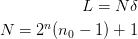
Unfortunately, it is not possible here to keep the physical scaling constant: either the physical volume does not remain fixed (shown) from level to level, or the points do not remain constant. When asking for abscissa through x(), the abscissa are rescaled so that the volume remains fixed with
 as the left
ghost-point (not shown).
as the left
ghost-point (not shown).This apparent difficulty can be dealt with when the full Galerkin approximation is used to propagate the operators and states down and up the hierarchy.
- ‘periodic’:
The grid consists of the following:
o       o       x     n=0  (n_0=2)
o   o   o   o   x     n=1
o o o o o o o o x     n=2
|----- L -------|

The periodic_center attribute changes this so that the center of the grid is at 0. Note that this means the different grids do not share the same abscissa values:
  x   o   x
  x o   o x
  xo o o ox
  |-------|
-L/2  0  L/2
- periodic_center
Center the periodic lattice.
Note
The centered lattice does not share common abscissa between the different grids.
- verbosity
10 for debugging, 20 for plotting - smoothing_algorithm
One of ‘GSLEX’ or ‘wJacobi’. See smooth_inplace(). - smoothing_weight
Weight for smoothing algorithm as a fraction of the default. Default is 1 for ‘GSLEX’ (the weight is not adjustable yet) and 2/3 for ‘wJacobi’. See smooth_inplace(). - preconditioner
‘gerschgorin’,‘abs_diagonal’, ‘Ditself’, None - sparse_solver
‘cgs’,‘bicgstab’, ‘cg’, ‘gmres’, ‘lgmres’ - sparse_solver_iterations
Counts the iterations used bythe sparse solver - current_state_dir
If this is defined, then the current state will be saved in a module of this name. - try_linsolve
If True then attempt linsolve for the base case, else jump to LdU decomposition straightaway. Computed Variables: - _stencil
stencil.Stencil class for computing .- _interpolator
stencil.Interpolator class for interpolating/restricting. - _L
Columns give the axes of the full lattice. See T(). - _Linv
Inverse basis transformation. See T(). - X
Abscissa. - shape
Shape of grid. Excluded Variables: - mg_sparse_tol_factor
The Multigrid preconditioner has to be more accurate than the sparse solver by this factor. The factor is different for robust_solve() and robust_solve2(), and have been chosen after experimenting with tolerances. Methods
A(x[, D, scale_factor]) Return A(x) all_items() Return a list [(name, obj)] of (name, object) pairs containing all items available. archive(name) Return a string representation that can be executed to restore the object. archive_1([env]) Return (rep, args, imports). average(f) Return the average value of f over the unit cell count(x[, A, b]) dx([N]) Return (dx, x_lower) where N is the number of dx_inv([shape]) Return dx_inv where shape is the shape of the lattice, get_A([D, scale_factor]) Return the matrix A. get_MAop([D, scale_factor, M, Dprecon, ...]) Return the left preconditioned linear operator M*A. get_N([n, inverse]) Return the number of points in the n‘th lattice. get_mats([D, scale_factor]) Return (As, Is, Rs) where these are lists of the initialize(**kwargs) Calls __init__() passing all assigned attributes. integrate(f) Return the integral of f over the unit cell interpolate(b[, mask]) Return the interpolation of the array b. items([archive]) Return a list [(name, obj)] of (name, object) pairs where the mynorm(v) norm of a vevtor v reshape(*argv) Reshape arguments for processing. restrict(b[, mask]) Return the restriction of the array b. resume() Resume calls to __init__() from __setattr__(), return_Dprecon([D, preconditioner, ...]) Return a suitable generalized mass matrix Dprecon for robust_solve(b[, D, Dprecon, scale_factor, ...]) Return the solution to the problem: .. robust_solve2(b[, D, Dprecon, scale_factor, ...]) Return the solution to the problem: .. save_current_state(D, A, b, abs_tol, ...) Save the current state to file. smooth_inplace(x, b, A[, shape]) Smooth x in place for system A*x=b. solve_(b[, D, scale_factor, x, abs_tol, ...]) Return x, the solution to  where
wheresolve_using_preconditioner(b[, D, ...]) Return the solution to the problem: .. solver([D, scale_factor]) Return a MG_solver object that provides an suspend() Suspend calls to __init__() from volume() Return the volume of a unit cell. x([n]) Return the n’th set of grid points. Initialize stuff
Methods
A(x[, D, scale_factor]) Return A(x) all_items() Return a list [(name, obj)] of (name, object) pairs containing all items available. archive(name) Return a string representation that can be executed to restore the object. archive_1([env]) Return (rep, args, imports). average(f) Return the average value of f over the unit cell count(x[, A, b]) dx([N]) Return (dx, x_lower) where N is the number of dx_inv([shape]) Return dx_inv where shape is the shape of the lattice, get_A([D, scale_factor]) Return the matrix A. get_MAop([D, scale_factor, M, Dprecon, ...]) Return the left preconditioned linear operator M*A. get_N([n, inverse]) Return the number of points in the n‘th lattice. get_mats([D, scale_factor]) Return (As, Is, Rs) where these are lists of the initialize(**kwargs) Calls __init__() passing all assigned attributes. integrate(f) Return the integral of f over the unit cell interpolate(b[, mask]) Return the interpolation of the array b. items([archive]) Return a list [(name, obj)] of (name, object) pairs where the mynorm(v) norm of a vevtor v reshape(*argv) Reshape arguments for processing. restrict(b[, mask]) Return the restriction of the array b. resume() Resume calls to __init__() from __setattr__(), return_Dprecon([D, preconditioner, ...]) Return a suitable generalized mass matrix Dprecon for robust_solve(b[, D, Dprecon, scale_factor, ...]) Return the solution to the problem: .. robust_solve2(b[, D, Dprecon, scale_factor, ...]) Return the solution to the problem: .. save_current_state(D, A, b, abs_tol, ...) Save the current state to file. smooth_inplace(x, b, A[, shape]) Smooth x in place for system A*x=b. solve_(b[, D, scale_factor, x, abs_tol, ...]) Return x, the solution to wheresolve_using_preconditioner(b[, D, ...]) Return the solution to the problem: .. solver([D, scale_factor]) Return a MG_solver object that provides an suspend() Suspend calls to __init__() from volume() Return the volume of a unit cell. x([n]) Return the n’th set of grid points. - __init__(*varargin, **kwargs)
Initialize stuff
- A(x, D=None, scale_factor=None)
Return A(x)
- average(f)
Return the average value of f over the unit cell (average).
- count(x, A=None, b=None)
- dx(N=None)
Return (dx, x_lower) where N is the number of points in the lattice, dx ` is the matrix who’s columns are the unit cell unit vectors and `x_lower is the coordinate of the lower corner.
- dx_inv(shape=None)
Return dx_inv where shape is the shape of the lattice, dx ` is the inverse of the matrix `dx who’s columns are the unit cell unit vectors.
- get_A(D=None, scale_factor=None)
Return the matrix A.
Parameters : D : array, optional
Array defining
 .
.scale_factor : array, optional
Array defining scale factors for the derivative term.
- get_MAop(D=None, scale_factor=None, M=None, Dprecon=None, maxiter_preconditioning_cycle=100, return_M=False, use_multigrid=True, abs_tol=None, rel_tol=None, seed_mg=False)
Return the left preconditioned linear operator M*A. This function is to be used as follows. If we want to solve for
 such that
  and know of a
preconditioning operator
and know of a
preconditioning operator  , then it may be easier to solve for
 .
.Parameters : M : sp.sparse.linalg.LinearOperator (optional)
There are three ways to specify the preconditioner. Firstly, we check if the preconditioner is explicitly specified as a linear operator.
Dprecon : array (optional)
Otherwise we check if the Dprecon matrix is given. If yes, then we generate Aprecon which can be inverted using multigrid.
- get_N(n=None, inverse=False)
Return the number of points in the n‘th lattice.
- get_mats(D=None, scale_factor=None)
Return (As, Is, Rs) where these are lists of the matrices required for Galerkin consistency.
Parameters : D : array, optional
Array defining
.scale_factor : array, optional
Array defining scale factors for the derivative term.
- integrate(f)
Return the integral of f over the unit cell (includes volume).
- interpolate(b, mask=None)
Return the interpolation of the array b.
Parameters : b : array
 . This is the only input required and is the
right-hand side for the i’th problem.
. This is the only input required and is the
right-hand side for the i’th problem.mask : array, optional
If specified, then only those dimensions where mask is True will be interpolated, otherwise all spatial dimensions will be interpolated.
Examples
>>> N = 15
>>> y1 = np.array([[1.0, 2, -1]])
>>> yd = np.ones((4,3,3,3))    # Test normalization with this
>>> m = MG(d=1, boundary_conditions='periodic')
>>> m.interpolate(y1)
array([[ 1. ,  1.5,  2. ,  0.5, -1. ,  0. ]])
>>> N = m.x().shape[1]
>>> m.interpolate(np.zeros((3, N))).shape, 2*N
((3, 32), 32)
>>> m.d = 3
>>> abs(m.interpolate(yd) - 1).max()
0.0
>>> m = MG(d=1, boundary_conditions='Neumann')
>>> m.interpolate(y1)
array([[ 1. ,  1.5,  2. ,  0.5, -1. ]])
>>> N = m.x().shape[1]
>>> m.interpolate(np.zeros((3, N))).shape, 2*(N-1) + 1
((3, 17), 17)
>>> m.d = 3
>>> abs(m.interpolate(yd) - 1).max()
0.0
- mynorm(v)
norm of a vevtor v
- reshape(*argv)
Reshape arguments for processing.
Usage:
x = self.reshape(x)
x, m, D = self.reshape(x, m, D)
Parameters : x : None
Inputs of None are passed through.
x : float
Floats are converted to an array of constants with shape (n,) + (N,)*d. If all arguments are scalars then it is assumed that n = 1.
x : array
Arrays are reshaped to either (n,) + (N,)*d (vector) or (n,n) + (N,)*d (matrix). If a matrix is included, then there must also be at least one vector argument otherwise everything will be assumed to be a vector.
When a matrix is reshaped as (n,n,N,N,...), the larger arrays must have the structure that the first two indices must be a matrix. This is consistent with forming D as a block matrix as show below.
Examples
>>> mg = MultiGrid(n=0, n_0=2, d=1)
>>> mg.reshape(1)
array([[ 1.,  1.]])
>>> mg.reshape(1,2,None)
[array([[ 1.,  1.]]), array([[ 2.,  2.]]), None]
>>> mg.reshape(1,[1, 2, 3, 4])
[array([[ 1.,  1.],
       [ 1.,  1.]]), array([[1, 2],
       [3, 4]])]
>>> mg = MultiGrid(n=0, d=2)
>>> f0 = np.sin(mg.x()[0])
>>> f1 = np.cos(mg.x()[0])
>>> f = np.array([f0,f1]).ravel()
>>> m = np.array([f0,f1]).ravel()
>>> D = np.array([[f0,f1],[2*f1,2*f0]])
>>> f_, m_, D_ = mg.reshape(f, m, D)
>>> np.allclose(f_[0,::], f0)
True
>>> np.allclose(f_[1,::], f1)
True
>>> np.allclose(m_[0,::], f0)
True
>>> np.allclose(m_[1,::], f1)
True
>>> np.allclose(D_[0,0,::], f0)
True
>>> np.allclose(D_[0,1,::], f1)
True
>>> np.allclose(D_[1,0,::], 2*f1)
True
>>> np.allclose(D_[1,1,::], 2*f0)
True
- restrict(b, mask=None)
Return the restriction of the array b.
Parameters : b : array
. This is the only input required and is the
right-hand side for the i’th problem.mask : array, optional
If specified, then only those dimensions where mask is True will be restricted, otherwise all spatial dimensions will be restricted.
Examples
>>> m = MG(d=1, n_0=3, boundary_conditions='periodic')
>>> y = np.array([[0., 1, 2, -3, 5, -1]])
>>> m.restrict(y)
array([[ 0.  ,  0.5,  1.5]])
>>> y = np.ones((4,6,6,6))    # Test normalization
>>> m.d = 3
>>> abs(m.restrict(y) - 1).max()
0.0
>>> m = MG(d=1, n_0=3, boundary_conditions = 'Neumann')
>>> y = np.array([[0., 1, 2, -3, 5]])
>>> m.restrict(y)
array([[ 0.25,  0.5 ,  1.75]])
- return_Dprecon(D=None, preconditioner=None, scale_factor=None, rel_tol=None)
Return a suitable generalized mass matrix Dprecon for which a multigrid preconditioner solving

can be used as a preconditioner to solving the real problem:
.. math::
left(-mat{s}nabla^2 + mat{D}) cdot x = bThe preconditioned mass term is made sufficiently definite that the multigrid algorithm will converge.
- robust_solve(b, D=None, Dprecon=None, scale_factor=None, preconditioner=None, use_multigrid=True, maxiter_sparse_solve=None, maxiter_preconditioning_cycle=100, maxiter_f_cycle=10, sparse_solver=None, abs_tol=None, rel_tol=None, seed_mg=False)
Return the solution to the problem:
Parameters : b : array
This must have no augmented structure unless D is also specified. This function assumes that all the elements of b are of the same order. I.e., the calling function ensures that the entries of b are scaled properly. But it doesnot assume that ||b|| is of the order of 1. We rescale b so that it is of the order 1.
scale_factor : array (optional)
Set of scale factors defining
 .
.Notes
This will always try to solve to the given max(rel_tol, abs_tol). abs_tol is supposed to be in units of b.
- robust_solve2(b, D=None, Dprecon=None, scale_factor=None, preconditioner=None, use_multigrid=True, maxiter_sparse_solve=None, maxiter_preconditioning_cycle=100, maxiter_f_cycle=10, sparse_solver=None, abs_tol=None, rel_tol=None, mg_rel_tol=None, mg_abs_tol=None, seed_mg=False)
Return the solution to the problem:
Parameters : b : array
This must have no augmented structure unless D is also specified. This function assumes that all the elements of b are of the same order. I.e., the calling function ensures that the entries of b are scaled properly. But it doesnot assume that ||b|| is of the order of 1. We rescale b so that it is of the order 1.
scale_factor : array (optional)
Set of scale factors defining
.Notes
This will always try to solve to the given max(rel_tol, abs_tol). abs_tol is supposed to be in units of b. The main differences from robust_solve are:
- It can take Dprecon as an input.
- It directly solves for M*A*x = M*b (where M is the preconditioning
operator, rather than give M as a preconditioning operator to the sparse solver.
- save_current_state(D, A, b, abs_tol, rel_tol, scale_factor)
Save the current state to file.
- smooth_inplace(x, b, A, shape=None)
Smooth x in place for system A*x=b.
Parameters : x : array
This must be a contiguous one-dimensional array. It will be smoothed in place.
b : array
Right-hand side.
A : csr_matrix
Matrix (should be in scipy.sparse.csr_matrix format for efficiency).
shape : tuple or None, optional
If shape = (d, n) is provided, then A is assumed to have block structure (d,n,d,n) and the diagonal portions of each block are explicitly solved for. Thus, for each equation, we partition:
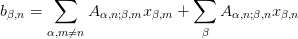
and solve for
 as
as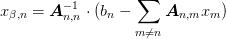
where
![\mat{A}_{m,n}[\alpha,\beta] = A_{\alpha,m;\beta,n}](../../../_images/math/42ce6c6aa191a8f880a7684ec871581a9119140f.png) .
.Notes
The following methods are implemented:
- ‘wJacobi’ : Weighted Jacobi method. This uses the diagonal
of
 as a preconditioner as well as a weight. The
full Jacobi step uses
as a preconditioner as well as a weight. The
full Jacobi step uses  (smoothing_weight) so
that the overall weight is 1, but this does not smooth very
well, hence the default overall weight is 2/3.
(smoothing_weight) so
that the overall weight is 1, but this does not smooth very
well, hence the default overall weight is 2/3.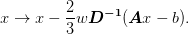
>>> np.random.seed(0)
>>> mg = MG(d=3, n=3, smoothing_algorithm='wJacobi')
>>> A = mg.get_mats()[0][-1]
>>> b = np.random.random(mg.shape)
>>> x = np.random.random(mg.shape)
>>> y = 1*x
>>> mg.smooth_inplace(x, b, A)
>>> y -= ((2./3*(A*y.ravel() - b.ravel())/A.diagonal()).
...       reshape(y.shape))
>>> np.allclose(x, y)
True
- ‘GSLEX’ : Lexicographic Gauss-Seidel. This algorithm makes
two sweeps through the data in lexicographic ordering solving each equation in the given system using the previous solutions (by updating x in place). Let
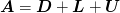 be decomposed into
diagonal and triangular pieces. One sweep goes down,
corresponding to the iteration:
be decomposed into
diagonal and triangular pieces. One sweep goes down,
corresponding to the iteration:
The second sweep corresponds to

The combined method is thus:
Note that if
 is symmetric, then
 and so
  , so the
combination of up and down sweeps maintains the symmetry.
, so the
combination of up and down sweeps maintains the symmetry.>>> np.random.seed(0) >>> mg = MG(d=3, n=3, smoothing_algorithm='GSLEX') >>> A = mg.get_mats()[0][-1] >>> b = np.random.random(mg.shape) >>> x = np.random.random(mg.shape) >>> y = 1*x >>> mg.smooth_inplace(x, b, A) >>> L = np.tril(A.toarray(), k=0) # Has diagonal piece L + D >>> U = np.triu(A.toarray(), k=0) # Has diagonal piece U + D >>> y -= np.linalg.solve(L, A*y.ravel()-b.ravel()).reshape(y.shape) >>> y -= np.linalg.solve(U, A*y.ravel()-b.ravel()).reshape(y.shape) >>> np.allclose(x, y) True
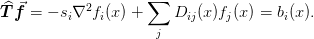
- solve_(b, D=None, scale_factor=None, x=None, abs_tol=None, rel_tol=None, max_iter=100)
Return x, the solution to
where![\mat{A} = -\mat{S}\op{\nabla}^2 + \mat{D}\\
A_{xy,ab} = - s_{a}[\op{\nabla}^2]_{xy} + D_{ab,x}](../../../_images/math/d0581e2ed317fba65939a13c2e23be5995b12744.png)
This iterates _f_cycle() until convergence is achieved.
Parameters : b : array
Array of the right hand side for the final lattice. The smaller arrays will be obtained by simply sampling this.
Represents a function evaluated over the abscissa satisfying the differential equation. If this is a vector valued function, then the latter dimensions should correspond to the underlying grid.
Valid dimensions are b.shape == (n, N, N, N,...) = (n,) + (N,)*d. The latter indices are over the d dimensions while the front index is over the auxiliary space. The first dimension may be neglected if there is no auxiliary space.
D : array, optional
This is a generalization of the mass matrix for cases where x represents a vector values function. D is a matrix in the extra co-ordinates, but must be diagonal in the grid (and hence only has one set of grid indices)
If provided, D must have shape d.shape = (n, n, N, N, N,...) = (n,)*2 + (N,)*d. I think there is a typo above. D has to have `d.shape = (n, n, N*d
= (n,)*2 + (N*d,)`.
scale_factor : array, optional
Array
 defining scale factors for the derivative term
.
defining scale factors for the derivative term
.x : array, optional
Initial guess. If provided, the multigrid cycle will be applied to the residual. Must have same shape as b.
abs_tol : float, optional
Optional override for abs_tol.
rel_tol : float, optional
Optional override for rel_tol.
max_iter : int, optional
Maximum number of iterations.
Examples
>>>
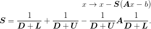
- solve_using_preconditioner(b, D=None, scale_factor=None, preconditioner=None, use_multigrid=True, Dprecon=None, maxiter_sparse_solve=None, sparse_solver=None, maxiter_preconditioning_cycle=100, sparse_solver_rel_tol=None, sparse_solver_abs_tol=None, abs_tol=None, rel_tol=None, seed_mg=False)
Return the solution to the problem:
Parameters : b : array
This must have no augmented structure unless D is also specified. This function assumes that all the elements of b are of the same order. I.e., the calling function ensures that the entries of b are scaled properly. But it doesnot assume that ||b|| is of the order of 1. We rescale b so that it is of the order 1.
scale_factor : array (optional)
Set of scale factors defining
.Notes
This will always try to solve to the given sparse_solver_rel_tol. The suggested sparse_solver_rel_tol is 100*rel_tol
- solver(D=None, scale_factor=None)
Return a MG_solver object that provides an f_cycle and v_cycle operation.
- volume()
Return the volume of a unit cell.
- x(n=None)
Return the n’th set of grid points. The ordering depends on the boundary conditions:
- Neumann:
In order to be consistent with a symmetric and charge-conserving Laplacian, the ghost-points must occur with a distance
. This leads to the
following arrangements. We take the left ghost point as
zero:x o o x n=0 (n_0 = 2) x o o o x n=1 x o o o o o x n=2 |-----------------------------| 0 L
- Periodic:
The left-most point of the unit cell is zero:
o       x
o   o   x
o o o o x
|-------|
0       L
The periodic_center attribute changes this so that the center of the grid is at 0:
x o x x o o x xo o o ox |——-|-L/2 0 L/2
Examples
>>> m = MG(d=2, n=0, n_0=5, L=5,
...        boundary_conditions='periodic',
...        periodic_center=True)
>>> x, y = m.x()
>>> np.allclose(x, np.fliplr(x)), np.allclose(y, np.flipud(y))
(True, True)
>>> x[:,0], y[0,:]
(array([-2., -1., 0., 1., 2.]), array([-2., -1., 0., 1., 2.]))
>>> m.periodic_center =  False
>>> x, y = m.x()
>>> np.allclose(x, np.fliplr(x)), np.allclose(y, np.flipud(y))
(True, True)
>>> x[:,0], y[0,:]
(array([ 0., 1., 2., 3., 4.]), array([ 0., 1., 2., 3., 4.]))
>>> m = MG(d=3, n=0, n_0=5, L=5, boundary_conditions='Neumann')
>>> x, y, z = m.x()
>>> x[:2,0,0], y[0,:2,0], z[0,0,:2]
(array([ 0.5,  1.5]), array([ 0.5,  1.5]), array([ 0.5,  1.5]))
- class mmf.math.multigrid.DivergenceError
Bases: exceptions.Exception
Raised if the f_cycle fails to reduce the residual, signaling a divergence.
- __init__()
x.__init__(...) initializes x; see help(type(x)) for signature
- class mmf.math.multigrid.WignerSeitz(*varargin, **kwargs)
Bases: mmf.objects.StateVars
This class sets up the spherical Wigner-Seitz approximation to problems of the form
WignerSeitz(mg=Required,
            n=Required,
            sparse_solver_iterations=0,
            verbosity=15,
            print_iter_frequency=1)
T
Attributes
State Variables: - mg
MultiGrid object. A multigrid cell to be approximated by a spherical Wigner-Seitz cell. - n
n for the Wigner Seitz multigrid. self.mgWS.n - sparse_solver_iterations
Number of sparse solver iterations - verbosity
Verbosity. - print_iter_frequency
Print every iteration divisible by this. Computed Variables: - R
The radius of the Wigner-Seitz cell. - mgWS
MultiGrid object. A Wigner-Seitz cell that approximates a given multigrid cell. - stencil_d2r
The stencil used for d^2 f/d r^2. - stencil_dr
The stencil used for d f/ dr. - stencil_0
The stencil used for getting the contribution for D!=0. - d
mg.d. - ls_r
mgWS.x()[0]. - C_d
The volume is C_d*R**d. - S_d
The surface area is S_d*R**(d-1). - r_tiny
Used to regulate 1/r by replacing it with 1/np.sqrt(r**2+r_tiny**2). Methods
A_sphericalWS(x[, D, scale_factor]) Return A(x) all_items() Return a list [(name, obj)] of (name, object) pairs containing all items available. archive(name) Return a string representation that can be executed to restore the object. archive_1([env]) Return (rep, args, imports). average(f) returns the integral of the field f divided count(x, sparse_solver[, A, b]) discretized_volume() returns the volume of the discretized hypershpere. get_A_sphericalWS([D, scale_factor]) Return the matrix A`=:math:-scale_factor*nabla^2+D`. We write A get_MAopWS(isolver[, D, scale_factor, M, ...]) Return the left preconditioned linear operator M*A. get_d_dr([D, scale_factor]) Return the matrix g`=:math:`d f/d r. initialize(**kwargs) Calls __init__() passing all assigned attributes. items([archive]) Return a list [(name, obj)] of (name, object) pairs where the resume() Resume calls to __init__() from __setattr__(), return_DpreconWS([D, preconditioner, ...]) Return a suitable generalized mass matrix Dprecon for solve_using_preconditionerWS(b, sparse_solver) Return the solution to the problem: .. suspend() Suspend calls to __init__() from volume() returns the volume of the hypershpere. - __init__(*varargin, **kwargs)
- A_sphericalWS(x, D=None, scale_factor=None)
Return A(x)
- average(f)
returns the integral of the field f divided by the volume.
Examples
Testing average of r**2 in 1, 2, 3d
>>> import mmf.math.multigrid._multigrid as multigrid_
>>> import numpy, scipy
>>> mg = multigrid_.MG(boundary_conditions='periodic',
...                d=3, n=4, n_0=(2, 2, 2), L=1.0)
>>> ws = multigrid_.WignerSeitz(mg=mg, n=mg.n)
>>> ls_r = ws.mgWS.x()[0]
>>> ls_f = ls_r**2
>>> assert(np.allclose(ws.average(ls_f), (3.0/5)*ws.R**2, atol=1e-3))
>>> mg = multigrid_.MG(boundary_conditions='periodic',
...                d=2, n=4, n_0=(2, 2), L=1.0)
>>> ws = multigrid_.WignerSeitz(mg=mg, n=mg.n)
>>> ls_r = ws.mgWS.x()[0]
>>> ls_f = ls_r**2
>>> assert(np.allclose(ws.average(ls_f), (2.0/4)*ws.R**2, atol=1e-3))
>>> mg = multigrid_.MG(boundary_conditions='periodic',
...                d=1, n=4, n_0=(2, ), L=1.0)
>>> ws = multigrid_.WignerSeitz(mg=mg, n=mg.n)
>>> ls_r = ws.mgWS.x()[0]
>>> ls_f = ls_r**2
>>> assert(np.allclose(ws.average(ls_f), (1.0/3)*ws.R**2, atol=1e-3))
- count(x, sparse_solver, A=None, b=None)
- discretized_volume()
returns the volume of the discretized hypershpere. Examples ——– Testing volume in 1, 2, 3d
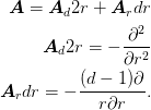
- get_A_sphericalWS(D=None, scale_factor=None)
Return the matrix A`=:math:-scale_factor*nabla^2+D`. We write A for a spherical Wigner-Seitz cell in d-dimensions as follows.
Parameters : D : array, optional
Array defining
.scale_factor : array, optional
Array defining scale factors for the derivative term.
Examples
Testing d^2 /dr^2
>>> import mmf.math.multigrid._multigrid as multigrid_
>>> import numpy, scipy
>>> mg = multigrid_.MG(boundary_conditions='Neumann',
...                d=3, n=3, n_0=(2, 2, 2), L=1)
>>> ws = multigrid_.WignerSeitz(mg=mg, n=mg.n)
>>> assert(np.allclose(
...                (np.pi**(mg.d/2.0)/scipy.special.gamma(1+mg.d/2.0))
...                *(ws.R**mg.d), (2**mg.d)*mg.volume() ))
>>> ls_r = ws.mgWS.x()[0]
>>> ls_V = 1/np.sqrt(ls_r**2+ws.r_tiny**2)
>>> A = ws.get_A_sphericalWS()
>>> assert(np.allclose((A*ls_V)[1:-1], 0, atol=1e-3))
>>> mg = multigrid_.MG(boundary_conditions='Neumann',
...                d=2, n=5, n_0=(2, 2), L=1)
>>> ws = multigrid_.WignerSeitz(mg=mg, n=mg.n)
>>> assert(np.allclose(
...                (np.pi**(mg.d/2.0)/scipy.special.gamma(1+mg.d/2.0))
...                *(ws.R**mg.d), (2**mg.d)*mg.volume() ))
>>> ls_r = ws.mgWS.x()[0]
>>> ls_V = scipy.log(np.sqrt(ls_r**2+ws.r_tiny**2/1000.0))
>>> #ls_V = 1/np.sqrt(ls_r**2+ws.r_tiny**2)
>>> A = ws.get_A_sphericalWS()
>>> #assert(np.allclose((A*ls_V)[1:-1], 0, atol=1e-3))
>>> #This is not a good test for small r.
- get_MAopWS(isolver, D=None, scale_factor=None, M=None, Dprecon=None, return_M=False, abs_tol=None, rel_tol=None, maxiter_precon=None)
Return the left preconditioned linear operator M*A. This function is to be used as follows. If we want to solve for
such that and know of a
preconditioning operator , then it may be easier to solve for
.Parameters : M : sp.sparse.linalg.LinearOperator (optional)
There are three ways to specify the preconditioner. Firstly, we check if the preconditioner is explicitly specified as a linear operator.
Dprecon : array (optional)
Otherwise we check if the Dprecon matrix is given. If yes, then we generate Aprecon which can be inverted using multigrid.
- get_d_dr(D=None, scale_factor=None)
Return the matrix g`=:math:`d f/d r. We write g for a spherical Wigner-Seitz cell in d-dimensions as follows.
Parameters : D : array, optional
Array defining
.scale_factor : array, optional
Array defining scale factors for the derivative term.
Examples
Testing d/dr
>>> import mmf.math.multigrid._multigrid as multigrid_
>>> mg = multigrid_.MG(boundary_conditions='periodic',
...   d=1, n_0=(2,), n=4, L=1)
>>> ws = multigrid_.WignerSeitz(mg=mg, n=mg.n)
>>> ls_r = ws.mgWS.x()[0]
>>> ls_V = np.cos(ls_r*2*np.pi)
>>> ls_dV = -2*np.pi*np.sin(ls_r*2*np.pi)
>>> A = ws.get_d_dr()
>>> dr = ws.mgWS.dx()[0][0,0]
>>> assert(np.allclose( A*ls_V/ls_dV, (np.sin(dr*2*np.pi)/(dr*2*np.pi)
...   *np.ones(ws.mgWS.shape)) ))
>>> ls_f = np.zeros((1, ) + ls_r.shape)
>>> ls_f[0, :] = scipy.exp(-ls_r**4/4)
>>> D = np.zeros((1, 1) + ls_r.shape)
>>> D[0, 0, :] = ls_r**3
>>> A = ws.get_d_dr(D=D)
>>> assert(np.allclose((A*ls_f.ravel())[:-1], 0, atol=1e-3))
- return_DpreconWS(D=None, preconditioner=None, scale_factor=None, rel_tol=None)
Return a suitable generalized mass matrix Dprecon for which a multigrid preconditioner solving
can be used as a preconditioner to solving the real problem:
.. math::
left(-mat{s}nabla^2 + mat{D}) cdot x = bThe preconditioned mass term is made sufficiently definite that the multigrid algorithm will converge.
- solve_using_preconditionerWS(b, sparse_solver, D=None, Dprecon=None, scale_factor=None, preconditioner=None, maxiter_sparse=None, maxiter_precon=None, rel_tol=None, abs_tol=None, preconditioner_abs_tol=None, preconditioner_rel_tol=None)
Return the solution to the problem:
Parameters : b : array
This must have no augmented structure unless D is also specified. This function assumes that all the elements of b are of the same order. I.e., the calling function ensures that the entries of b are scaled properly. But it doesnot assume that ||b|| is of the order of 1. We rescale b so that it is of the order 1.
scale_factor : array (optional)
Set of scale factors defining
.Notes
This will always try to solve to the given sparse_solver_rel_tol. The suggested sparse_solver_rel_tol is 100*rel_tol
- volume()
returns the volume of the hypershpere. Examples ——– Testing volume in 1, 2, 3d
>>> import mmf.math.multigrid._multigrid as multigrid_
>>> import numpy, scipy
>>> mg = multigrid_.MG(boundary_conditions='periodic',
...                d=3, n=3, n_0=(2, 2, 2), L=1.0)
>>> ws = multigrid_.WignerSeitz(mg=mg, n=mg.n)
>>> assert(np.allclose(ws.volume(), (4.0/3)*numpy.pi*(ws.R)**3))
>>> mg = multigrid_.MG(boundary_conditions='periodic',
...                d=2, n=3, n_0=(2, 2), L=1.0)
>>> ws = multigrid_.WignerSeitz(mg=mg, n=mg.n)
>>> assert(np.allclose(ws.volume(), numpy.pi*(ws.R)**2))
>>> mg = multigrid_.MG(boundary_conditions='periodic',
...                d=1, n=3, n_0=(2, ), L=1.0)
>>> ws = multigrid_.WignerSeitz(mg=mg, n=mg.n)
>>> assert(np.allclose(ws.volume(), 2*(ws.R)))