Two delta-x wave in the ACOM3 model

Two delta-x wave in the ACOM3 model


Links to other pages:

     1a. TAO/model comparisons
     1b. Model exploration 1 (E Pacific mixing)
     2.   Model Exploration 2 (Other things)
     3.   Model Exploration 3 (circ E of Australia)
     4.   Two-delta-x wave?    (This page)
     5.   Throughflow XBT lines

     6.   Writeup


This page brings together plots, some of which are also on other pages, illutrating the 2 delta-x wave in the ACOM3 model. All these plots were made with file subdomain_new (model with tides).
The problem has come up in several areas, most clearly in attempting to find the total transport across the Pacific Equator, in which wildly inflated results were found using the file sample_new (see plots under the heading "Cross-equatorial transport in ACOM3 sliced different ways" about 2/3 of the way down another page).
      The problem was traced to a 2-delta-x oscillation in the meridional current, and the subsampling (every 4th point in x) hits all the peaks of one sign.
      What seems remarkable is that these oscillations are nearly steady, or while their amplitude may change their phase remains constant; as a result they are clearly seem in the mean v. Also remarkable is that they are much much less apparent in the zonal current.

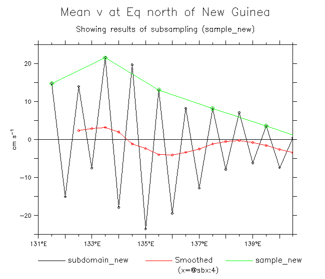
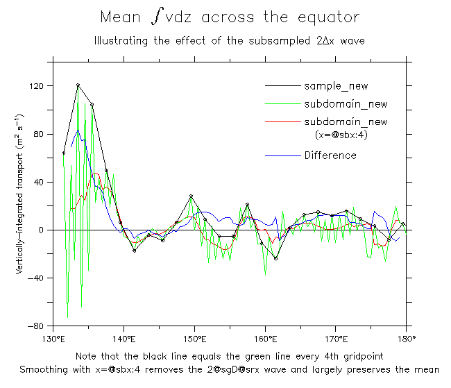
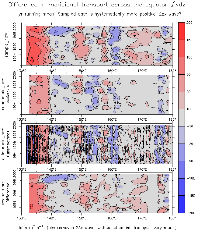
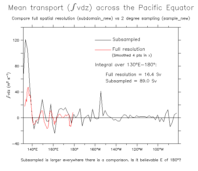
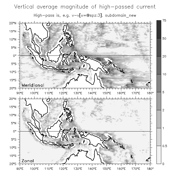
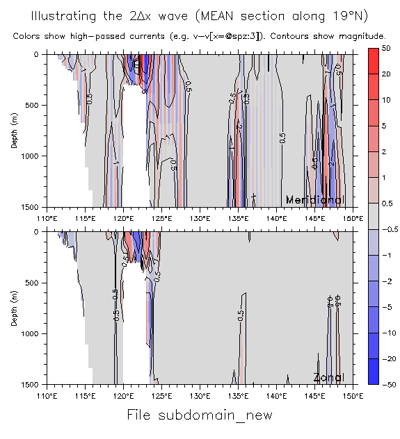
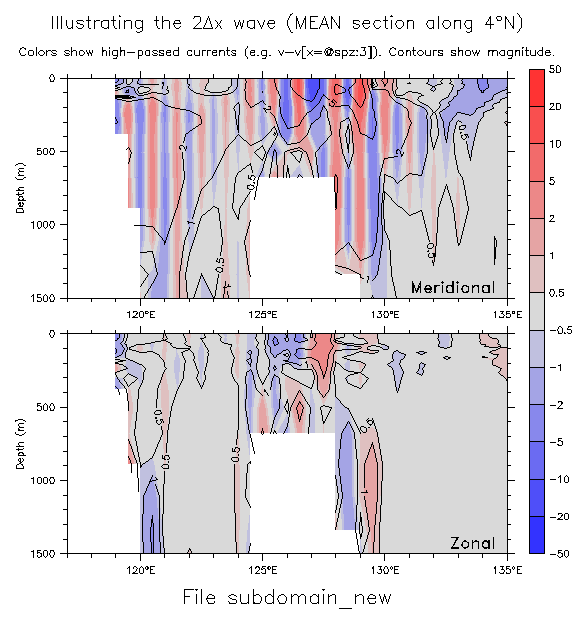
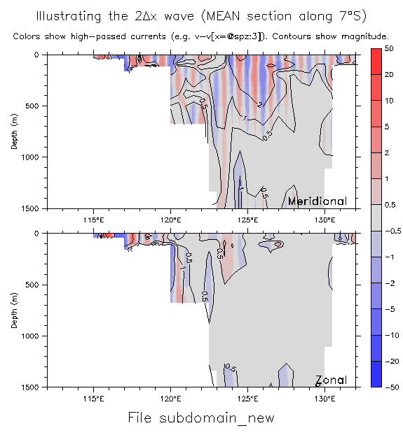
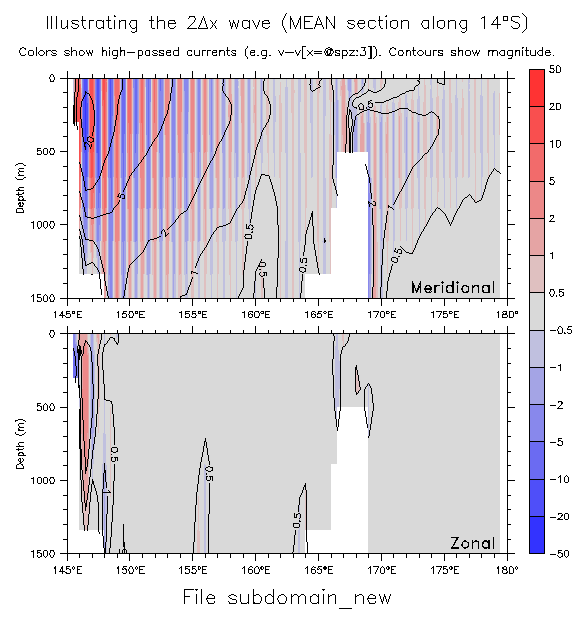
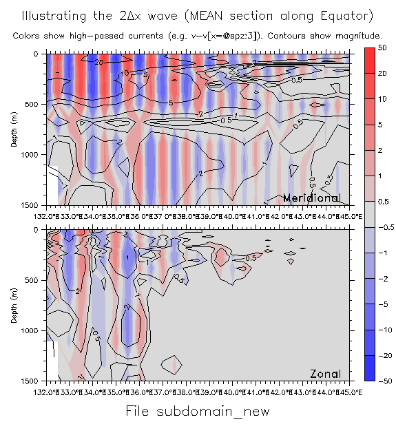
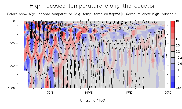
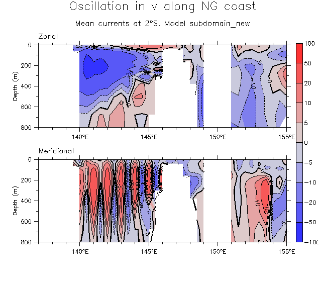
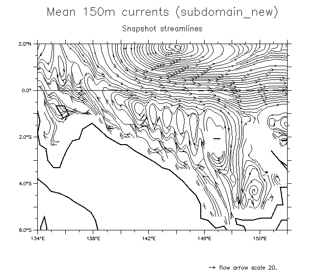
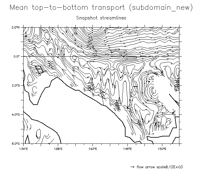
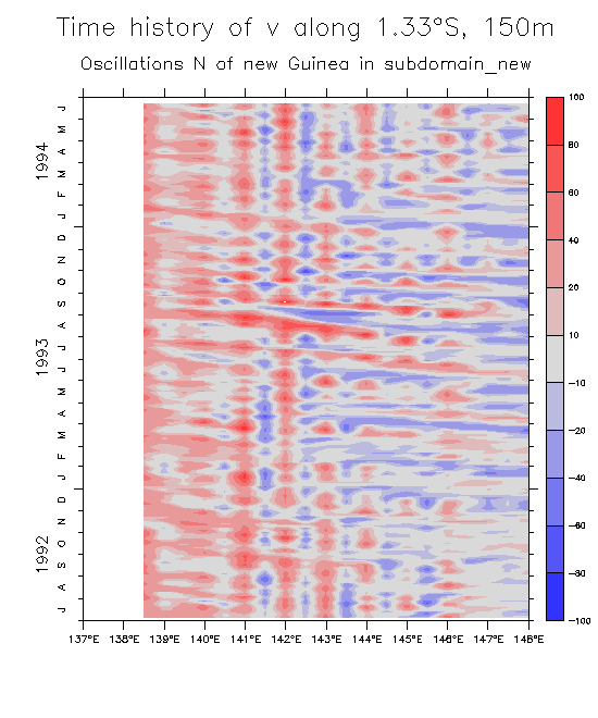
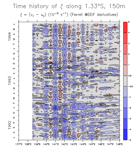
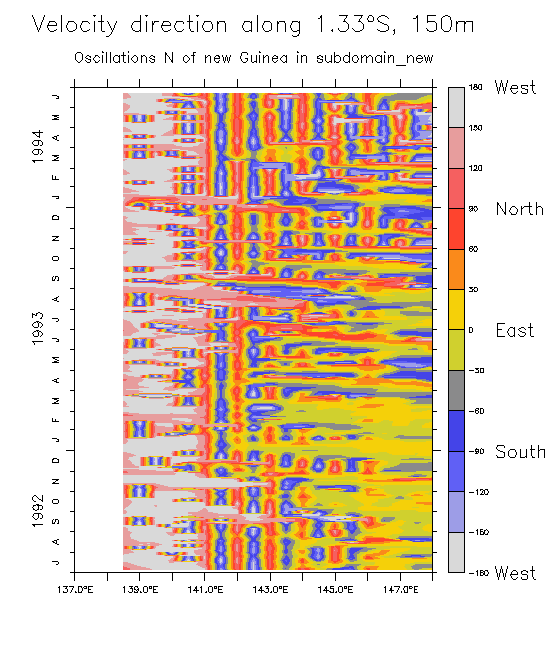
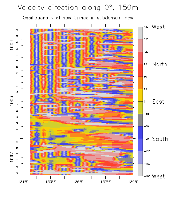
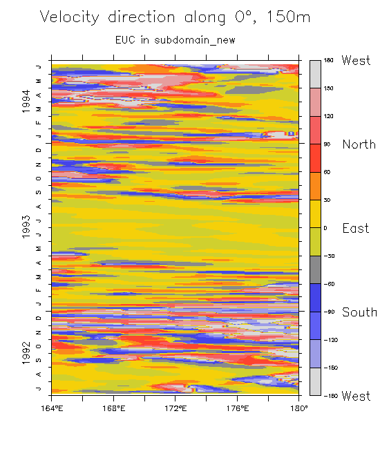
->  From these plots it seems clear that the oscillation is
1) related to strong currents near topography;
2) very much stronger in v than in u;
3) does not propagate;
4) only in x;
5) extends over large vertical distances;
6) can have phase reversals with depth;
7) only weakly related to temperature variations.

  1. v N of New Guinea     extended to 180°
  2. Time series of the difference show that it is systematically positive (by chance???), and that the oscillations are standing.
  3. The vertically-integrated transport between 130°E and 180° (where direct comparison is possible) is 89 Sv from subsampled data but 16.4 Sv from the full resolution data.

    Some exploration of the spatial distribution of this oscillation was done by high-pass filtering u and v (e.g. v-v[x=@spz:3]):

  4. Map of vertically-averaged magnitude of highpassed u and v
  5. Sections of high-passed u and v in likely locations:
    a. 19°N   4°N   Equator   7°S   14°S   
    b. Detail at equator shows reversal with depth
    c. Overlay high-passed temperature
    -> Note that corresponding plots checking for 2-delta-y oscillations are nearly blank.

  6. a. Another view of the difference between u and v   Sfc Streamlines
    b. Further details:  Surface   150m   Transport   
    c. Relative vorticity at 150m   
    d. Time history: 2°S:   v   Rel Vort   Current direction   Equator: Direction   Direction, EUC at 180° (for checking)