Solution of Problem IV with MATLAB using simultaneous solution for the conduction terms and Netwon-Raphson for the heat generation terms (Version 2).
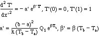
The problem to be solved is
The finite difference formulation of this problem is
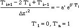
Henceforth the primes will be dropped for convenience. Rearrange the differential equation to the following form.
![]()
The Newton-Raphson method is applied to this set of equations. The nonlinear equations fi are expanded in a Taylor series about a known solution, Tik, and we neglect terms higher order than linear.
![]()
Since we want to find the new value such that the functions fi are zero, we set the left-hand side to zero.
![]()
Rearrange this to give
![]()
We rewrite this using a matrix, AA.
![]()
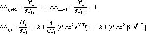
where
![]()
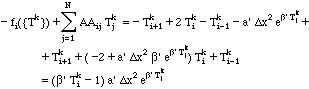
In other simulations of boundary value problems, the iterative scheme was set up with Tk+1 on one side, and Tk on the other. This is done here, which allows us to use the same the convergence test. The iterative scheme is then
![]()
where the superscript k represents the value of the quantity at the k-th iteration. Thus, one takes values at the k-th iteration and calculates the values with the superscript k+1. These values are then used in the equation again and again. The process repeats until the values no longer change, to within a specified tolerance specified by you.
In this case we have the following entries for the matrix AA.
The right-hand side will be
These equations are applied here using MATLAB for a' = 2, b' = 0.5. The command file is shown below.
%solution to Problem IV using Newton-Raphson
dx = 1;
beta=0.5;
for kk=1:5
dx = dx/2;
n = 1 + 1/dx
tol = 1e-12;
% set up initial guess
for i=1:n
y1(i) = dx*(i-1);
end
%begin iteration
change = 1.;
iter=0;
while change>tol
iter=iter+1;
sum = 0.;
% Compute the matrices.
for i=1:n
heat(i) = 2*dx*dx*exp(beta*y1(i));
end
for i=2:n-1
f(i) = (beta*y1(i)-1.)*heat(i);
for j=1:n
aa(i,j) = 0.;
end
aa(i,i-1) = 1;
aa(i,i) = -2+ beta*heat(i);
aa(i,i+1) = 1;
end
% The first and last rows are special.
f(1) = 0;
f(n) = 1;
aa(1,1) = 1;
aa(1,2) = 0;
aa(n,n-1) = 0;
aa(n,n) = 1;
% Solve for one iteration.
y2 = aa\f';
% Compute variables needed to test convergence
sum=0.;
for i=1:n
sum = sum + abs(y1(i) - y2(i));
y1(i) = y2(i);
end
change = sum
% Test to see that change < tol.
end
% Collect numbers for plotting.
nm = (n-1)/2 + 1
x=dx*(nm-1)
ys(kk) = y1(nm);
xs(kk) = dx*dx;
iters(kk)=iter
end
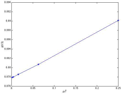
% Plot T(0.5) versus x^2.
plot(xs,ys,'-*')
xlabel('x^2')
ylabel('y(0.5)')
clear aa
clear f
clear y1
clear y2
ys
xs
iters
The program initially sets the tolerance, grid size, and number of points. Then the first guess for y(x) is taken as a straight line. The iteration will continue until change is less than the desired tolerance. Change is defined as
![]()
Sum is the cumulative sum of absolute values of the changes in y at each node. Finally, the new value, y2, is transferred to the old value, y1, and sum is transferred to change so that the 'while' change can be tested. Finally, the last few commands print the solution and number of iterations.
How do we check our work? First, we set heat(i) = 0, which is the same as taking the no heat generation. In that case the solution should be a straight line, and it is. If we need to troubleshoot, we remove the ';' from the statements, use delx = 0.25, and do the calculations by hand to compare with the MATLAB results. This insures that the calculations follow the equations given above. When we have a solution, we can take the values and substitute them into the equation they are supposed to satisfy. If they do, then the equations are satisfied. You have to use judgment to decide how many of the equations you need to test; it depends on how the MATLAB program is written. Next, we solve using successively smaller ∆x and see if the solution changes. The results are (for tolerance = 10-12):
| ∆x | y(0.5) | No. of iterations |
| 0.5 | 0.890152 | 4 |
| 0.25 | 0.880706 | 4 |
| 0.125 | 0.878543 | 4 |
| 0.0625 | 0.878013 | 4 |
| 0.03125 | 0.877882 | 4 |
The numbers are close to each other. Furthermore the increments between the answers are:
(0.5, 0.25): 0.890152 0.880706 = 0.0945
(0.25, 0.125): 0.880706 0.878543 = 0.00216
(0.125, 0.0625): 0.878543 0.878013 = 0.000533
(0.0625, 0.03125): 0.878013 - 0.877882 = 0.000131
The error should go as ∆x'2; with a ∆x half as big, the error should be one-fourth as big. If we are in the region (small enough ∆x') where this applies, the differences should decrease by a factor of 4 each time. In this case 0.000533 / 4 = 0.000134, which is close enough to say the convergence is followed. Extrapolation to zero gives T'(0.5) = 0.877836. The figure also shows convergence which is proportional to ∆x2.
Notice that this solution is also the same derived using Excel or the other version of MATLAB. That is as it should be, since we are solving the same equations. The only reason for a difference is that we might not have set the tolerance to a small enough value. Needless to say, the more accurate we want the solution, the smaller is the tolerance, and the more iterations we need. What is interesting is that with the Newton-Raphson method only 4 iterations were necessary to achieve a tolerance of 10-12, in contrast to the successive substitution method, which needed 18 or 19. The values of change for one ∆x were successively:
Change, for b' = 0.5, a' = 2, ∆x = 0.03125
7.91
0.102
2.03 x 10⁻⁵
6.97 x 10⁻¹³
The convergence is very rapid once the solution gets close to the final answer. This is a feature of the Newton-Raphson method.
This case is a particularly hard one to solve when b' is large. In fact, for the case ∆x = 0.5 it can be shown that a solution (real) does not exist for b' larger than 0.926111 (proof). You can try this value yourself and see what happens. This is an example that underscores the necessity to carefully check your program. If you had not done that, the logical assumption would be that you had made a mistake. However, if the program is carefully checked then the results can be depended upon. In this case, no solution is possible, but to know that requires other analysis (link).
How do we know the accuracy of our result? Firstly, we have run the problem with five different ∆x and find similar results. Secondly, we calculated the truncation error, found the error was proportional to ∆x2, and found that the results were also proportional to ∆x2 for the smallest ∆x. These two results confirm that we have solved some problem correctly. Thirdly, we carefully checked every line of the code and made sure that we solved the equation we intened to solve. Fourthly, we extrapolated the results in ∆x2 to zero to obtain the answer, 0.877836. Thus, the last calculation, with ∆x = 0.03125, was accurate to within 0.000046, or with 0.005% accuracy.
Take Home Message: The Newton-Raphson method (properly programmed!) solves this nonlinear problem fast and efficiently. The programming is more extensive, though.