Solution to Problem IV using Excel
The problem to be solved is Problem III.
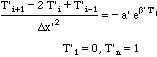
The finite difference formulation of this problem is
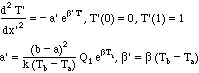
Henceforth the primes will be dropped for convenience. Rearrange the differential equation to the following form.
![]()
The iterative scheme can be represented as
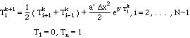
where the superscript k represents the value of the quantity at the k-th iteration. Thus, one takes values at the k-th iteration and calculates the values with the superscript k+1. These values are then used in the equation again, and again. The process repeats until the values no longer change, to within a specified tolerance specified by you. For a' = 2, b' = 0.5 the equation is
These equations are applied here using Microsoft Excel Spreadsheet, but the commands are generic ones that most spreadsheets allow. Consider the grid shown in the Figure.
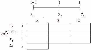
The first row is reserved for the value of y at each grid point. The left-most cell is the value of y at the first point, and the right-most cell is the value of y at the last point. Since these values are known we simply insert the known values in the cells. For the points in between, we insert the equation given above.
It is convenient if we define some quantities, first, though, to simplify the algebra. Let the second row represent the value of x at the node i. The value of ∆x is placed in cell A4; first use 0.5. The first value of x, 0, is placed in the cell A2. Then the equation is written in cell B2 and copied to the right.
B2: = A2+$A$4, copied to the right
The $A$4 insures that when the cell formula is copied to the right, the next cell has B2+$A$4, then C2+$A$4; in other words, the A4 location is absolute and is not incremented during the copying. Once this is done, the second row should show the values 0, 0.5, 1.0.
The heat generation term is placed in the third row. The first column uses:
A3: = $A$4*$A$4*exp(0.5*A1), copied to the right
Then the formulas for the cells involving yi are simply:
B1: = 0.5*(A1 + C1) + B3, copied to the right.
When you are placing these formulas in your spreadsheet, the program, will give you a warning since you are defining a circular reference, that is some cells are defined in terms of other cells, which are in tern defined in terms of the the first cells. To begin the calculation in Microsoft Excel you have to choose Tools, then Preferences, then Calculation, and check the Iteration Box. That tells the computer that you will be performing iterations. (You may wish to prepare the spreadsheet with 'Iteration' turned off and turn it on when preparation is complete. This will prevent getting weird answers during the preparation when all the cells are not complete. This is especially true for non-linear problems.) There you can also set the maximum number of iterations to 500, and the convergence parameter to 10-6. After you choose Calculate Now the spreadsheet should look like this.
| A | B | C | |
| 1 | 0 | 0.8901522 | 1.000000 |
| 2 | 0 | 0.5 | 1 | 3 | 0.25 | 0.3901522 | 0.4121803 |
| 4 | 0.5 |
How do we check our work? First, we make sure that the numbers we put in are correct. We check cell A4, which has the value of ∆x; 0.5 is correct. Then we check the second row, which shows the location of the grid points. They should be x = 0, 0.5, 1.0, and these are correct. We then check the third row. Since we copied the formula, we only need to check one cell. For cell B3 the value should be
![]()
and this checks as well. Lastly we check the cell B1. We can use the numbers in A1 and C1, since the cell formula does, too. We get
![]()
Since these calculations agree, we conclude we have set the spreadsheet up correctly. There is one final check that can be done. Notice in the formulas that if we set ∆x = 0, then the third row is all zero. This is equivalent to saying there is no heat generation. Under those circumstances the solution to the problem is a straight line. Set cell A4 to 0 and see. The second row is zero, too, but as long as the third row is zero, the second row is essentially not used. Since we get the straight line we have added confidence in our solution.
Next do the same thing with a ∆x = 0.25. The spreadsheet results are shown in the Table.
| A | B | C | D | E | |
| 7 | 0 | 0.5214707 | 0.8807059 | 1.045784 | 1 |
| 8 | 0 | 0.25 | 0.5 | 0.75 | 1 |
| 9 | 0.0625 | 0.0811178 | 0.0970785 | 0.105431 | 0.1030451 |
| 10 | 0.25 |
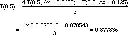
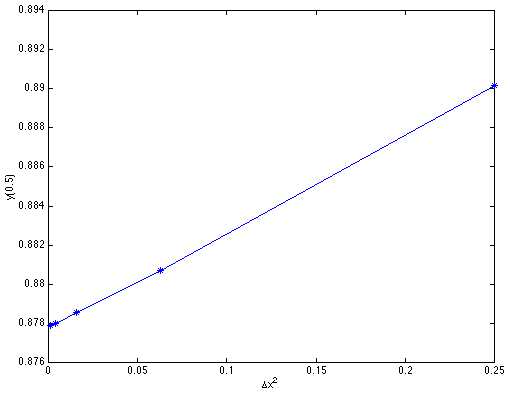
Note that the value at x = 0.5 is within 1% of the one derived using ∆x = 0.5. To be absolutely sure that the spreadsheet is prepared correctly, this spreadsheet is checked in the same way. Finally, use ∆x = 0.125, and then 0.0625. The answers obtained for T(0.5) are shown below (using a tolerance of 10-8).
| ∆x | y(0.5) |
| 0.5 | 0.890152 |
| 0.25 | 0.880706 |
| 0.125 | 0.878543 |
| 0.0625 | 0.878013 |
The numbers are close to each other. Furthermore the increments between the answers are:
(0.5, 0.25): 0.890152 0.880706 = 0.0945
(0.25, 0.125): 0.880706 0.878543 = 0.00216
(0.125, 0.0625): 0.878543 0.878013 = 0.000533
The error should go as ∆x2; with a ∆x half as big, the error should be one-fourth as big. If we are in the region (small enough ∆x) where this applies, the differences should decrease by a factor of 4 each time. In this case 0.00216 / 4 = 0.00054, which is close enough to say the convergence is followed. That is clear in the figure. We can also use The Richardson extrapolation to deduce the best value.
Notice that this solution is also the same derived using MATLAB, as it should be, since we are solving the same equations. The only reason for a difference is that we might not have set the tolerance to a small enough value. Needless to say, the more accurate we want the solution, the smaller is the tolerance, and the more iterations we need.
This case is a particularly hard one to solve when b' is large. In fact, for the case ∆x = 0.5 it can be shown that a solution (real) does not exist for b' larger than 0.926111 (proof). You can try this value in your spreadsheet and see what happens. Before doing so, turn off the calculation feature, fix the spreadsheet as you like, and then turn on the calculation feature. The calculations will quickly diverge, giving indeterminate results in the spreadsheet. This is an example that underscores the necessity to carefully check your spreadsheet. If you had not done that, the logical assumption would be that you had made a mistake. However, if the spreadsheet is carefully checked then the results can be depended upon. In this case, no solution is possible, but to know that requires other analysis (link).
Take Home Message: Spreadsheet programs can be used to solve the finite difference equations, but solutions may not exist for nonlinear problems, or they may be difficult to find.