Richardson extrapolation of finite difference methods.
Inthe finite difference method, a Richardson extrapolation can be used to improve the accuracy. Suppose we do a calculation with ∆x, getting a result, which we call here y1. This might be the value of the solution y at a specific position, x. Suppose the finite difference method we used has a truncation error that is proportional to ∆x2. Then let's write the exact answer, yex, in terms of the numerical results, y1 and ∆x.
![]()
The . . . represent terms we have ignored, since these are multiplied by powers of ∆x higher than 2, and these terms will be small when ∆x is small. We just calculated y1, and we know ∆x, so why don't we just calculate yex from this formula? We don't know C, thus we can't find yex. Furthermore, we don't know the . . .. Thus redo the problem, this time using a grid spacing of ∆x/2, i.e. using twice as many grid points. Call the solution, y2 , at the same specific position, x. Then let's write the exact answer, yex, in terms of the numerical results, y2 and ∆x.
![]()
We now have two unknowns, C and yex, and two equations. Solve them for C and yex.
![]() ,
, ![]()
Thus if we have a solution y1 obtained with grid spacing ∆x, and a solution y2 obtained with grid spacing ∆x/2, an improved solution is given by
![]()
This gives a good estimate provided ∆x is small enough that the method is truly a second order method, and the neglected terms are small.
The way to see if the neglected terms are small is to do a series of computations, each with ∆x half the size of the previous one, and see if the results can be represented as a straight line. To see the expected behavior, do another calculation with grid spacing ∆x/4, and call the result y3. Write the additional equation
![]()
Now combination of the three equations gives
This means that the difference between the third and second result is one-fourth of the difference between the second and first result. Thus, we can test whether the error is really proportional to ∆x2 by examining those differences. The increments between solutions should decrease by a factor of 4 each step. Alternatively, we can plot the result versus ∆x2, and it should be a straight line.
![]()
As an example of this theory, consider Problem II in the section on the finite difference method applied to boundary values (link). The table shows the result obtained for the center value of y when using various ∆x. These results are plotted in the Figure.
Values of y(0.5) for Finite Difference Method, Problem II
| ∆x | y(0.5) | Estimated Error |
| 0.5 | 0.59375 | 5.21E-03 |
| 0.25 | 0.58984375 | 1.30E-03 |
| 0.125 | 0.588867188 | 3.26E-04 |
| 0.0625 | 0.588623047 | 8.14E-05 |
| 0.03125 | 0.588562012 | 2.03E-05 |
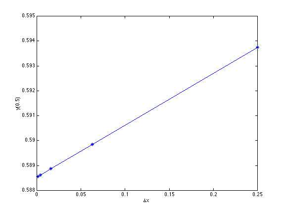
Solution to Problem II using the Finite Difference Method; plotted versus ∆x2
Clearly for small ∆x the plot becomes linear; this suggests that the ∆x is small enough that the theory applies, and the missing terms represented by . . . are negligible.
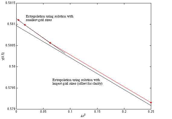
If the last two points are used extrapolate to zero the result is
![]()
The fact that the curve is linear versus ∆x2 for small ∆x is one sign that we have done the calculation correctly. It shows that we have successfully implemented a second-order finite difference method to some problem. Whether we have done this for the right problem must be tested in the method (see the examples provided with each method). Here we can also compare the answer with the exact solution, since it is known to be 0.5885416667. The extrapolated finite difference solution gives the same answer, which verifies that we have solved the correct problem. The solution with ∆x = 0.03125 has an actual error of 0.000020, but the extrapolated solution is exact to 10 digits. If we use the extrapolated answer to compute estimated errors of the solutions in the tables, we get the values listed and plotted below. Clearly the errors are proportional to ∆x2 and decrease by a factor of 4 at each step.

Estimated Error for Problem II using the Finite Difference Method
One might be tempted to use all the data and fit it with a straight line of y versus ∆x2. This is generally not recommended, however, because the data for larger ∆x have more error in them (the neglected terms . . . are bigger); thus less weight should be given those points in the extrapolation. Using the last two points, once one verifies the straight line, gives the most accurate results.
Another example of the same thing is for Problem III in the section on finite difference methods for boundary value problems.
Values of y(0.5) for Finite Difference Method, Problem III
| Ćx | y(0.5) | Estimated Error |
| 0.5 | 0.579156 | 1.98E-03 |
| 0.25 | 0.58056 | 5.78E-04 |
| 0.125 | 0.580986 | 1.52E-04 |
| 0.0625 | 0.5811 | 3.80E-05 |
Solution to Problem III using the Finite Difference Method; plotted versus ∆x2
A plot of y(0.5) shows that it is proportional to ∆x2; thus we can use the analysis. The extrapolated answer is then
![]()
The estimated errors are shown in the Table, too, and they decrease by a factor of about 4 each step, as they should. The actual value from the exact solution is 0.581139.
For the next example, use the results from Problem IV, which is a nonlinear problem without a known analytic solution. The results for the temperature at the mid-point were:
| Ćx | T(0.5) | Estimated Error |
| 0.5 | 0.890152 | 1.23E-02 |
| 0.25 | 0.880706 | 2.87E-03 |
| 0.125 | 0.878543 | 7.07E-04 |
| 0.0625 | 0.878013 | 1.77E-04 |
The figure shows that the results are linear in ∆x2.
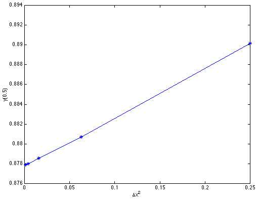
Solution to Problem IV using the Finite Difference Method; plotted versus ∆x2
Furthermore the increments between the answers are:
(0.5, 0.25): 0.890152 0.880706 = 0.0945
(0.25, 0.125): 0.880706 0.878543 = 0.00216
(0.125, 0.0625): 0.878543 0.878013 = 0.000533
The error should go as ∆x'2; with a ∆x half as big, the increments should be one-fourth as big, and this is the case. Using the last two values and the extrapolation formula gives the extrapolated answer:
T'(0.5) = (4 x 0.878543 0.878013 ) / 3 = 0.877836.
The estimated errors are made using this value, and they decrease by a factor of 4 each step, thus validating the analysis. In this case no exact solution is known, and we depend on this error analysis to tell the magnitude of the error in the computation.
The same analysis can be done when the order is different from 2. Let us do the analysis for a method whose truncation error is proportional to ∆xp. Do two calculations, one with ∆x and one with ∆x / 2; call the respective results y1 and y2. The expansions give
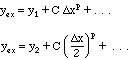
Solve these two equations for yex.
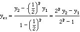
This is the extrapolation law for a method with truncation error proportional to ∆xp. It is instructive to write these out for several different orders.

Clearly, for the higher order methods, the correction is a smaller and smaller portion of the final result and the role of extrapolation is less useful.
Take Home Message: Improved accuracy can be obtained by solving the same problem with two different grid sizes and extrapolating the results to zero grid size.