Multiple Nonlinear Equations using the Newton-Raphson Method
For systems of equations the Newton-Raphson method is widely used, especially for the equations arising from solution of differential equations.
![]()
Write a Taylor expansion in several variables.
![]()
The Jacobian matrix is defined as
![]()
and the Newton-Raphson method is
![]()
Since the Jacobian depends on the iterate, it must be evaluated at each iteration. Sometimes the method converges even though the Jacobian is not reevaluated at each iteration. In this formulation of the method the right-hand side gradually (hopefully!) goes to zero. There are two alternate ways to write the Newton-Raphson method.
![]()
![]()
The first one of these is useful in theoretical developments (although an LU decomposition (link) is used rather than a matrix inverse (link)). The second one is such that upon convergence the right-hand side approaches a constant that doesn't change with further iterations.
Newton-Raphson method using MATLAB
Next let us apply the Newton-Raphson method to the system of two nonlinear equations solved above using optimization methods. The equations to solve are
![]()
and the Jacobian is
Prepare the following script (but without the ';' at the end of each line).
% Newton Raphson solution of two nonlinear algebraic equations
% set up the iteration
error1 = 1.e8;
xx(1) = 0; % initial guesses
xx(2) = 0;
iter=0;
maxiter=30.
% begin iteration
while error1>1.e-12
iter=iter+1;
x = xx(1);
y = xx(2);
% calculate the functions
f(1) = 10*x+3*y*y-3;
f(2) = x*x-exp(y) -2.;
% calculate the Jacobian
J(1,1) = 10;
J(1,2) = 6*y;
J(2,1) = 2*x;
J(2,2) = -exp(y);
% solve the linear equations
y = -J\f';
% move the solution, xx(k+1) - xx(k), to xx(k+1)
xx = xx + y';
% calculate norms
error1=sqrt(y(1)*y(1)+y(2)*y(2))
error(iter)=sqrt(f(1)*f(1)+f(2)*f(2));
ii(iter)=iter;
if (iter > itermax)
error1 = 0.;
s=sprintf('****Did not converge within %3.0f iterations.****',itermax);
disp(s)
end
% check if error1 < 1.e-12
end
x = xx(1);
y = xx(2);
f(1) = 10*x+3*y*y-3;
f(2) = x*x-exp(y) -2.;
% print results
f
xx
iter
% plot results
semilogy(ii,error)
xlabel('iteration number')
ylabel('norm of functions')
clear ii
clear error
The first three lines initialize three things. The initial conditions for x1 and x2 are set here, and the value of error is set here. The definition of error is

and we would like it to be zero. The M-file is structured so that the calculation in the while-end loop will continue indefinitely until error is less than 10-12. Thus the value of error is initially set to a large value, 108, so that this condition is not satisfied before beginning. (Some languages test the condition on entry, some on exit; to be safe assume both!)
Inside the while-end loop, the values of x1 and x2 are moved to local variables, which are easier to use in the statements following. Then the two functions are evaluated. Next the elements of the Jacobian are evaluated. The Newton-Raphson method uses
Jk ( xk+1 xk) = fk
If we let
y = xk+1 xk
then the Newton-Raphson method is
Jk y = fk
Likewise the value of xk+1 is
xk+1 = xk + y
Thus the next statements compute y and xk. Since we are not sure if this problem has a solution,
we will test 'error', which is the square root of the sum of the squares of the functions, which should be zero. If error < 10-12 then the loop ends; finally it computes f and prints it. Thus we find the solution x and the function f, which is to be zero. Note that we have to recalculate f with the latest value of x in order to find f for the last solution.
Before we can rely on the results, we must check the M-file carefully. First remove all the ';' so that the calculations are printed out as they are made. Change the initial values from [0,0] to [1.5, 2.5]. The functions should be 30.75 and -11.9325. Run the M-file (by issuing the command >nr and quickly press the apple-period. (Alternatively, insert the command 'pause' in the code where you would like to stop and look at the results.) Look at the results on the screen for the first time through the calculation. The values of f and the Jacobian are correct.
J11 =10, J12 = 15
J21 = 3, J22 = 12.1825
We already know that MATLAB solves the linear equations correctly, but watch that you have the minus sign! Now put back in the ';' and run the problem for as many iterations as it needs. (If it takes hundreds of iterations you probably made a mistake. Stop and check your work). The results are:
xx = 1.44555236880496 2.41215834803947
error = 8.953656560885539e-13
f =
1.0e-14 *
0.17763568394003 0
The solution has been found. The change in the solution from one iteration to another was less than 10-12, and the function itself is smaller than 10-14 for the first element and zero to machine accuracy for the second element. The iterative behavior is shown in the figure. It took about 20 iterations before the error started significant reductions, but once that point was reached the error decreased rapidly.
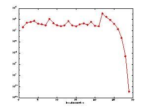
Figure NR2. Value of Error in the Newton-Raphson Method for Example II.
The successive substitution method did not work for this example.
Take Home Message: Convergence may not occur, but once the iterate is close, convergence is fast.