Derivation of Finite Difference Method for Problem IV.

Finally, solve Problem IV, which is a heat transfer problem.

Here we take the thermal conductivity, k, as a constant, and a heat generation rate that is exponential.

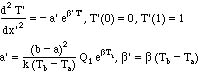
The full problem is then

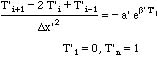
It is convenient to make the equations nondimensional (link). This is always good practice because some of the numbers may be of very different magnitude and can get lost in the calculation. Thus we introduce the nondimensional variables

and derive the following equation (link)

The finite difference method applied to these equations gives

Here we solve the equations for the parameters, a' = 2, b' = 0.5, using the same methods as before.

Matlab, using successive substitution (link)

Matlab, using Newton-Raphson (link)

Excel, using successive substitution (link)

Since we have solved Problem II already, and have verified our work, it is a small task to change to Problem IV. We do that and get the following results for the temperature at the mid-point.

∆x	y(0.5)
0.5	0.890152
0.25	0.880706
0.125	0.878543
0.0625	0.878013

The numbers are close to each other. Furthermore the increments between the answers are:

(0.5, 0.25): 0.890152 ­ 0.880706 = 0.0945

(0.25, 0.125): 0.880706 ­ 0.878543 = 0.00216

(0.125, 0.0625): 0.878543 ­ 0.878013 = 0.000533

The error should go as ∆x'²; with a ∆x' half as big, the error should be one-fourth as big. If we are in the region (small enough ∆x') where this applies, the differences should decrease by a factor of 4 each time. In this case 0.00216 / 4 = 0.00054, which is close enough to say the convergence is followed. That is clear in the figure.

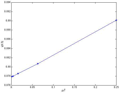
Figure BVP6. Solution to Problem IV using the Finite Difference Method; plotted versus ∆x²

Extrapolation (link) to zero gives T'(0.5) = 0.877836.

There are a number of complications that can make the problem even harder to solve.

geometry (link), variable mesh (link), BC explanation (link), derivative BC (link), heat flux derivation (link).