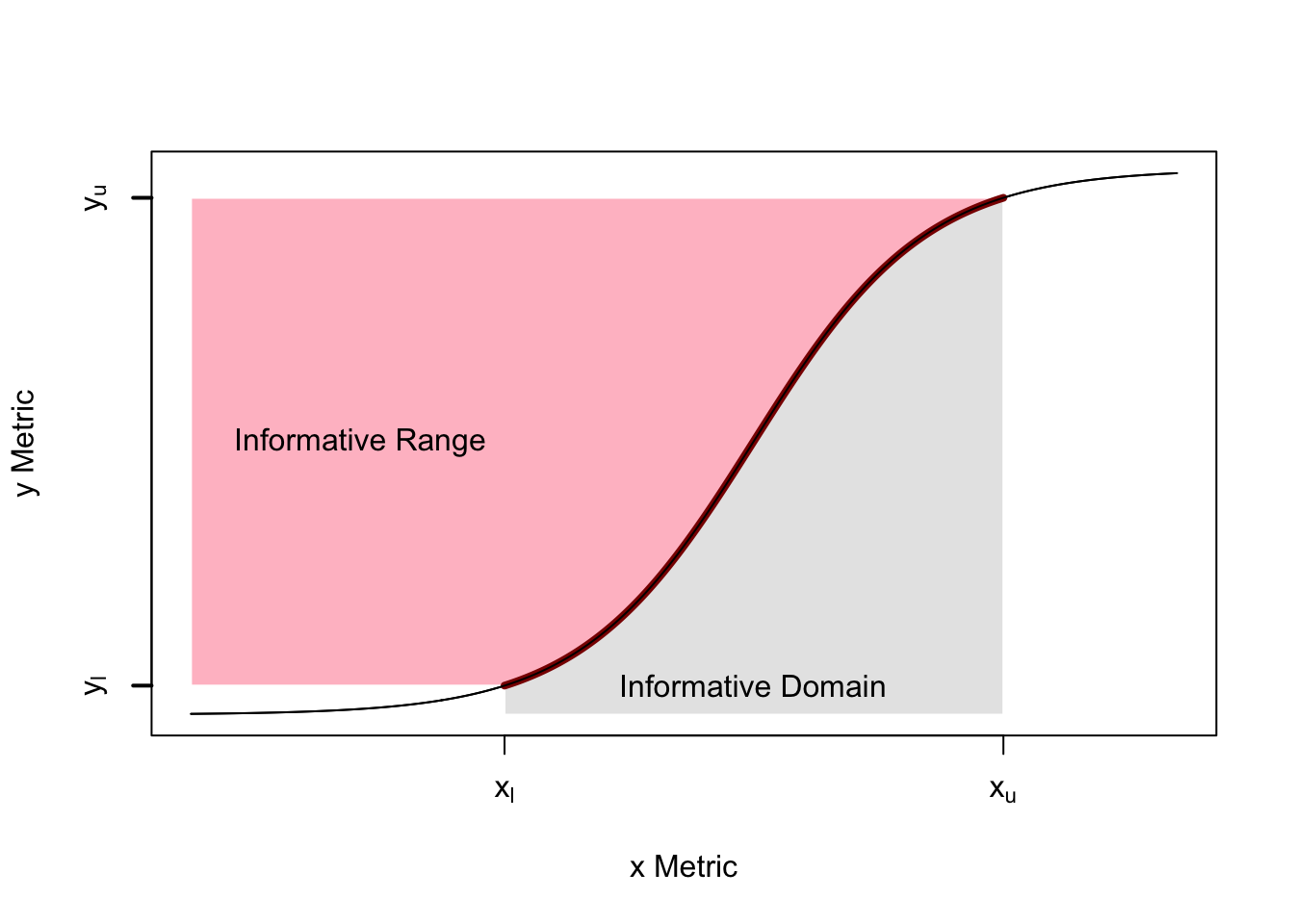
Informative Range

---

We define the informative range as a way of understanding the amount of information conveyed about one variable through a non-linear relationships with another.

---

Definition

For any relationship between two variables \(x\) and \(y\) where \[y = f(x) + \epsilon,\] where \(\epsilon\) represents noise. Let \(y\) be the variable we want to predict using information about \(x.\) The informative range for prediction is a subset of the full range, \(y \in (y_l, y_u)\) with corresponding values in the informative domain for \(x \in (x_l, x_u).\) We define a the informative range and domain by defining a cutoff on the slope, \(f'(x) > \phi,\) so that we get enough information about \(y\) around values of around \(x\) to get information about \(y\) that we can trust.

---

Figure: An illustration of the informative range and domain for a sigmoidal relationship with no noise.

---

Lines

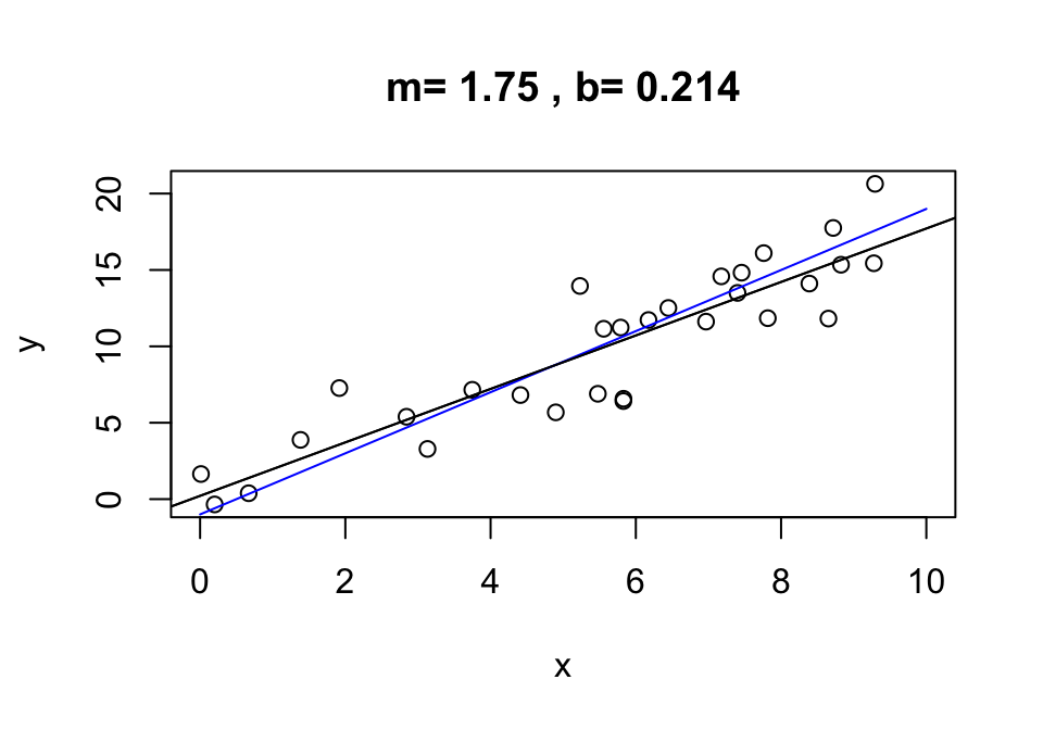
If the relationship between two variables is linear, then information about one variable is equally informative about another across its entire range. For example, if we have the fitted relationship for a set of points

\[y = f(x) + \epsilon = mx + b + \epsilon\]

then \(f'(x)=m,\) So the relative amount of information about \(y\) is constant across the entire range of \(x.\) We can thus \(x\) to predict \(y\) and vice versa.

In the following, if we accept that the fitted relationship is the true relationship (a reasonable but risky assumption; in this case, the true value was \(m=2\)), we know that a one unit change in \(x\) will result in an expected 7/4 unit change in \(y\). We can, moreover, use \(y\) to predict \(x\):

\[x \approx \frac{y-b + \epsilon}{m}\]

so a one unit change in \(y\) will result in an expected \(4/7\) change in \(x\). Notably, the error scales with \(1/m\).

---

Figure 2: For linear relationships, the amount of information about \(y\) does not change across values of \(x.\)

Sigmoidal Relationships

If the relationship between two variables is sigmoidal, then the amount of information about the variable \(y\) depends on the value of \(x\):

\[y = \frac{1}{1 + e^{-S(x-d)}} + \epsilon\] In the following example, we let \(d=10\) and \(S=1.2.\)

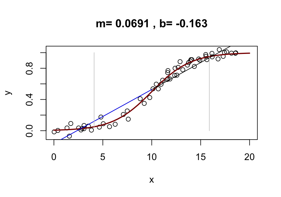
We note that the greatest change in \(y\) is found when \(x\) is around \(d=10\). Since the range of \(y \in c(0,1)\), about 90% of the total variance in y occurs for \(x\in c(4.11, 15.889).\)

c(sigmoidF(10+ll, .5, 10), sigmoidF(10-ll, .5, 10))

[1] 0.9500029 0.0499971

In this case, we can write down a closed form expression for the change in \(y\) by looking at the derivative of the sigmoidal function:

\[ \frac{S e^{-S(x-d)}}{(1-e^{-S(x-d)})^2}\]

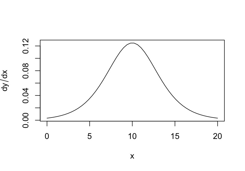
Around \(x=10\), a one-unit change in \(x\) will result in a maximum 12% change in \(y\), but as we move away from the peak, the amount of information about \(y\) from \(x\) declines.

---

The right way to do prediction is probably to try and fit a sigmoidal curve to the data.

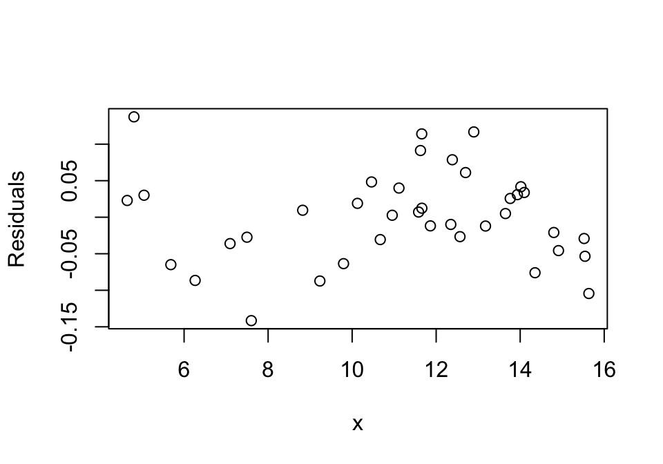
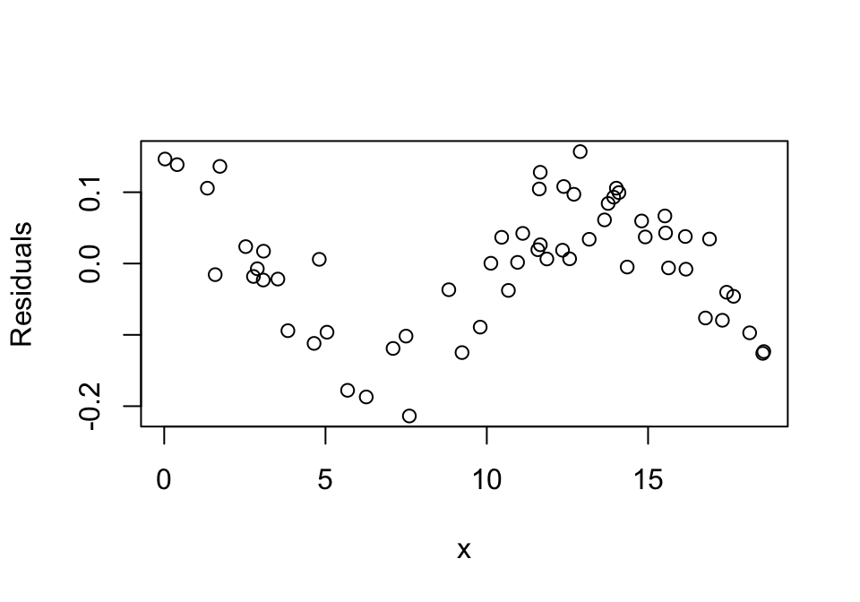
We note that the fitted line provides a poor fit by visual inspection of the residuals. Since the residual error should be uniformly distributed with no pattern, we can also see how bad we’ve done by plotting the residuals:

If, however, we include only values of \(x\) that contain 90% of the range of \(y\), we get a reasonably good linear fit, to the true relationship. The 9% slope from the fitted line is about 3/4 of the maximum 12% slope predicted above.

Call:
lm(formula = ysub ~ xsub)

Residuals:
      Min        1Q    Median        3Q       Max 
-0.141548 -0.034737  0.003852  0.033085  0.137366 

Coefficients:
             Estimate Std. Error t value Pr(>|t|)    
(Intercept) -0.396674   0.037822  -10.49 1.71e-12 ***
xsub         0.090297   0.003258   27.71  < 2e-16 ***
---
Signif. codes:  0 '***' 0.001 '**' 0.01 '*' 0.05 '.' 0.1 ' ' 1

Residual standard error: 0.0634 on 36 degrees of freedom
Multiple R-squared:  0.9552,    Adjusted R-squared:  0.954 
F-statistic: 768.1 on 1 and 36 DF,  p-value: < 2.2e-16

If we plot the residuals, it’s hard to tell the relationship within the subsetted data are not linear.