9 Week 9

Topic: Miscellaneous data processing

This week's lesson will cover a set of miscellaneous data processing topics.

Mostly this is a set of coded examples with explanations

9.1 Substituting text

9.1.1 paste(), paste0()

Pasting text allows you to substitute variables within a text string. For example, if you are running a long loop over a series of files and you want to know which file name and loop iteration you are on.

The function paste() combines a set of strings and adds a space between the strings, e.g., combining the first values from the LETTERS and the letters built-in vectors:

paste(LETTERS[1], letters[1])

## [1] "A a"

whereas paste0 does not add spaces:

paste0(LETTERS[1], letters[1])

## [1] "Aa"

Download the file quickfox to an arbitrary location on your computer. The code below assumes it was stored in C:/Users/phurvitz/AppData/Local/Temp.

# a temp location--get dirname of dirname of the tempdir
tmp <- tempdir() %>%
    dirname()
# zip file
zipfile <- file.path(tmp, "quickfox.zip")
# unzip
unzip(zipfile = zipfile, overwrite = TRUE, exdir = tmp)
# files in the zipfile
fnames <- unzip(zipfile = file.path(tmp, "quickfox.zip"), list = TRUE) %>%
    pull(Name) %>%
    file.path(tmp, .)

# read each file
for (i in seq_len(length(fnames))) {
    # the file name
    fname <- fnames[i]
    # read the file
    mytext <- scan(file = fname, what = "character", quiet = TRUE)

    # vvvvvvvvvvvvvvvvvvvvvvvvvvvvvv
    # make a string using `paste()`
    mystr <- paste(mytext, "    ", i, "of", length(fnames), fname)
    # ^^^^^^^^^^^^^^^^^^^^^^^^^^^^^^

    # print the message
    message(mystr)
}

## the      1 of 9 C:/Users/phurvitz/AppData/Local/Temp/str_0017e602b137e88.txt

## quick      2 of 9 C:/Users/phurvitz/AppData/Local/Temp/str_0027e604fa83778.txt

## brown      3 of 9 C:/Users/phurvitz/AppData/Local/Temp/str_0037e60bc634af.txt

## fox      4 of 9 C:/Users/phurvitz/AppData/Local/Temp/str_0047e60195772f.txt

## jumps      5 of 9 C:/Users/phurvitz/AppData/Local/Temp/str_0057e60229c264.txt

## over      6 of 9 C:/Users/phurvitz/AppData/Local/Temp/str_0067e606cfd4207.txt

## the      7 of 9 C:/Users/phurvitz/AppData/Local/Temp/str_0077e601b5b742d.txt

## lazy      8 of 9 C:/Users/phurvitz/AppData/Local/Temp/str_0087e604c1a30c5.txt

## dog      9 of 9 C:/Users/phurvitz/AppData/Local/Temp/str_0097e6038323213.txt

9.1.2 sprintf()

sprintf() can be used to format text. Here are just a few examples. The result is a formatted text string.

9.1.2.1 Formatting numerical values

Leading zeros

Numeric values can be formatted with a specific number of decimal places or leading zeros. For example, ZIP codes imported from CSV files often are converted to integers. The following code chunk converts some numerical ZIP code-like values to text values with the correct format.

Bad ZIP codes:

# some numerical ZIP codes
(zip_bad <- data.frame(id = 1:3, zipcode = c(90201, 02134, 00501)))

##   id zipcode
## 1  1   90201
## 2  2    2134
## 3  3     501

Good ZIP codes:

# fix them up
(zip_good <- zip_bad %>% mutate(
    zipcode = sprintf("%05d", zipcode)
))

##   id zipcode
## 1  1   90201
## 2  2   02134
## 3  3   00501

Decimal places

Numerical values with different numbers of decimal places can be rendered with a specific number of decimal places.

# numers with a variety of decimal places
v <- c(1.2, 2.345, 1e+5 + 00005)

# four fixed decimal places
v %>% sprintf("%0.4f", .)

## [1] "1.2000"      "2.3450"      "100005.0000"

Note that this is distinct from round(), which results in a numeric vector:

# round to 4 places
v %>% round(., 4)

## [1]      1.200      2.345 100005.000

9.1.2.2 String substitutions

sprintf() can also be used to achieve the same substitution in the file reading loop above. Each %s is substituted in order of the position of the arguments following the string. Also note that \t inserts a TAB character.

# read each file
for (i in seq_len(length(fnames))) {
    # the file name
    fname <- fnames[i]
    # read the file
    mytext <- scan(file = fname, what = "character", quiet = TRUE)

    # vvvvvvvvvvvvvvvvvvvvvvvvvvvvvv
    # make a string using `paste()`
    mystr <- sprintf("%s\t%s of %s:\t%s", mytext, i, length(fnames), fname)
    # ^^^^^^^^^^^^^^^^^^^^^^^^^^^^^^

    # print the message
    cat(mystr)
}

## the  1 of 9: C:/Users/phurvitz/AppData/Local/Temp/str_0017e602b137e88.txtquick   2 of 9: C:/Users/phurvitz/AppData/Local/Temp/str_0027e604fa83778.txtbrown   3 of 9: C:/Users/phurvitz/AppData/Local/Temp/str_0037e60bc634af.txtfox  4 of 9: C:/Users/phurvitz/AppData/Local/Temp/str_0047e60195772f.txtjumps    5 of 9: C:/Users/phurvitz/AppData/Local/Temp/str_0057e60229c264.txtover 6 of 9: C:/Users/phurvitz/AppData/Local/Temp/str_0067e606cfd4207.txtthe 7 of 9: C:/Users/phurvitz/AppData/Local/Temp/str_0077e601b5b742d.txtlazy    8 of 9: C:/Users/phurvitz/AppData/Local/Temp/str_0087e604c1a30c5.txtdog 9 of 9: C:/Users/phurvitz/AppData/Local/Temp/str_0097e6038323213.txt

9.1.3 str_replace(), str_replace_all()

The stringr functions str_replace() and str_replace_all() can be used to substitute specific strings in other strings. For example, we might create a generic function to run over a set of subject IDs that generates a file for each subject.

subjects <- c("a1", "b2", "c3")

f <- function(id) {
    # create an output filename by substituting in the subject ID
    outfname <- "C:/temp/xIDx.csv" %>% str_replace(pattern = "xIDx", id)
    # ... do a bunch of stuff, for example
    val <- rnorm(1)
    # write the file
    message(paste0("writing"))
    write.csv(x = val, file = outfname)
}

for (i in subjects) {
    f(i)
}

## writing
## writing
## writing

9.2 Showing progress

A text-based progress bar can be shown using txtProgressBar(). Here we run the same loop for reading the text files, but rather than printing the loop iteration and file names, we show the progress bar and the file contents. If no text is printed to the console (unlike what is demonstrated below with cat()), the progress bar will not print on several lines.

n_fnames <- length(fnames)
# create progress bar
pb <- txtProgressBar(min = 0, max = n_fnames, style = 3)

## 
  |                                                                                                              
  |                                                                                                        |   0%

for (i in 1:n_fnames) {
    # delay a bit
    Sys.sleep(0.1)
    # update progress bar
    setTxtProgressBar(pb, i)
    # read and print from the file
    txt <- scan(fnames[i], what = "character", quiet = TRUE)
    cat("\n", txt, "\n")
}

## 
  |                                                                                                              
  |============                                                                                            |  11%
##  the 
## 
  |                                                                                                              
  |=======================                                                                                 |  22%
##  quick 
## 
  |                                                                                                              
  |===================================                                                                     |  33%
##  brown 
## 
  |                                                                                                              
  |==============================================                                                          |  44%
##  fox 
## 
  |                                                                                                              
  |==========================================================                                              |  56%
##  jumps 
## 
  |                                                                                                              
  |=====================================================================                                   |  67%
##  over 
## 
  |                                                                                                              
  |=================================================================================                       |  78%
##  the 
## 
  |                                                                                                              
  |============================================================================================            |  89%
##  lazy 
## 
  |                                                                                                              
  |========================================================================================================| 100%
##  dog

close(pb)

9.3 Turning text into code: eval(parse(text = "some string"))

Sometimes you may have variables whose values that you want to use in a command or function. For example, suppose you wanted to write a set of files, one for each ZIP code in a data frame, with a file name including the ZIP code. We would not want to use the column name zipcode, but we want the actual value.

We can generate a command using some kind of text substitution as above with sprintf()

for (i in zip_good %>% pull(zipcode)) {
    # do some stuff
    vals <- rnorm(n = 3)
    y <- bind_cols(zipcode = i, v = vals)
    # a writing command using sprintf() to substitute %s = ZIP code
    cmd <- sprintf("write.csv(x = y, file = 'C:/temp/%s.csv', row.names = FALSE)", i)

    # this runs the command
    eval(parse(text = cmd))
}

9.4 SQL in R with RSQLite and sqldf

Sometimes R's syntax for processing data can be difficult and confusing. For programmers who are familiar with structured query language (SQL), it is possible to run SQL statements within R using a supported database back end (by default SQLite) and the sqldf() function.

For example, the mean sepal length by species from the built-in iris data set can be obtained, presented in Table 9.1

library(sqldf)

sqlc <- 'select 
    "Species" as species
    , avg("Sepal.Length") as mean_sepal_length
from iris
group by "Species";
'

iris_summary <- sqldf(x = sqlc)

iris_summary %>% 
    kable(caption = "Mean sepal length from the iris data set") %>% 
    kable_styling(full_width = FALSE, position = "left")

Table 9.1: Mean sepal length from the iris data set

species	mean_sepal_length
setosa	5.006
versicolor	5.936
virginica	6.588

9.5 Downloading files from password-protected web sites

Some web sites are protected by simple username/password protection. For example, try opening [http://staff.washington.edu/phurvitz/csde502_winter_2021/password_protected] (http://staff.washington.edu/phurvitz/csde502_winter_2021/password_protected). The username/password pair is csde/502, which will allow you to see the contents of the web folder.

If you try downloading the file through R, you will get an error because no password is supplied.

try(
    read.csv("http://staff.washington.edu/phurvitz/csde502_winter_2021/password_protected/foo.csv")
)

##   id zipcode
## 1  1    2134

However, the username and password can be supplied as part of the URL, as below. When the username and password are supplied, they will be cached for that site for the duration of the R session.

try(
    read.csv("http://csde:502@staff.washington.edu/phurvitz/csde502_winter_2021/password_protected/foo.csv")
)

##   id zipcode
## 1  1    2134

9.6 Dates and time stamps: POSIXct and lubridate

R uses POSIX-style time stamps, which are stored internally as the number of fractional seconds from January 1, 1970. It is imperative that the control over time stamps is commensurate with the temporal accuracy and precision your data. For example, in the measurement of years of residence, precision is not substantially important. For measurement of chemical reactions, fractional seconds may be very important. For applications such as merging body-worn sensor data from GPS units and accelerometers for estimating where and when physical activity occurs, minutes of error can result in statistically significant mis-estimations.

For example, you can see the numeric value of these seconds as options(digits = 22); Sys.time() %>% as.numeric().

options(digits = 22)
Sys.time() %>% as.numeric()

## [1] 1615062338.7390621

If you have time stamps in text format, they can be converted to POSIX time stamps, e.g., the supposed time Neil Armstrong stepped on the moon:

(eagle <- as.POSIXct(x = "7/20/69 10:56 PM", tz = "CST6CDT", format = "%m/%d/%y %H:%M"))

## [1] "1969-07-20 10:56:00 CDT"

Formats can be specified using specific codes, see strptime().

The lubridate package has a large number of functions for handling date and time stamps. For example, if you want to convert a time stamp in the current time zone to a different time zone, first we get the current time

library(lubridate)

## 
## Attaching package: 'lubridate'

## The following objects are masked from 'package:base':
## 
##     date, intersect, setdiff, union

# set the option for fractional seconds
options(digits.secs = 3)
(now <- Sys.time() %>% strptime("%Y-%m-%d %H:%M:%OS"))

## [1] "2021-03-06 12:25:39.028 PST"

And convert to UTC:

# show this at time zone UTC
(with_tz(time = now, tzone = "UTC"))

## [1] "2021-03-06 20:25:39.028 UTC"

or show in a different format:

# in different format
now %>% format("%A, %B %d, %Y %l:%m %p %Z")

## [1] "Saturday, March 06, 2021 12:03 PM PST"

9.7 Timing with Sys.time() and difftime()

It is easy to determine how long a process takes by using sequential Sys.time() calls, one before and one after the process, and getting the difference with difftime(). For example,

# mark time and run a process
t0 <- Sys.time()
Sys.sleep(5)
t1 <- Sys.time()

# difftime() unqualified will make its best decision about what to print
(difftime(time1 = t1, time2 = t0))

## Time difference of 5.155155 secs

# time between moon step and now-ish
(difftime(time1 = t0, time2 = eagle))

## Time difference of 18857.19 days

difftime() can also be forced to report the time difference in the units of choice:

(difftime(time1 = t1, time2 = t0, units = "secs") %>% as.numeric()) %>% round(0)

## [1] 5

(difftime(time1 = t1, time2 = t0, units = "mins") %>% as.numeric()) %>% round(2)

## [1] 0.09

(difftime(time1 = t1, time2 = t0, units = "hours") %>% as.numeric()) %>% round(4)

## [1] 0.0014

(difftime(time1 = t1, time2 = t0, units = "days") %>% as.numeric()) %>% round(6)

## [1] 6e-05

9.8 Faster files with fst()

The fst package is great for rapid reading and writing of data frames. The format can also result in much smaller file sizes using compression. Here we will examine the large Add Health file. First, a download, unzip, and read as necessary:

library(fst)

## fst package v0.9.4

## (OpenMP detected, using 4 threads)

myUrl <- "http://staff.washington.edu/phurvitz/csde502_winter_2021/data/21600-0001-Data.dta.zip"
# zipfile in $temp
tmp <- tempdir() %>% dirname()
zipfile <- file.path(tmp, basename(myUrl))
# dta file in $temp
dtafname <- tools::file_path_sans_ext(zipfile)
# check if the dta file exists
if (!file.exists(dtafname)) {
    # if the dta file doesn't exist, check for the zip file
    # check if the zip file exists, download if necessary
    if (!file.exists(zipfile)) {
        curl::curl_download(url = myUrl, destfile = zipfile)
    }
    # unzip the downloaded zip file
    unzip(zipfile = zipfile, exdir = Sys.getenv("TEMP"))
}

# read the file
dat <- read_dta(dtafname)

# save as a CSV, along with timing
t0 <- Sys.time()
csvfname <- dtafname %>% str_replace(pattern = "dta", replacement = "csv")
write.csv(x = dat, file = csvfname, row.names = FALSE)
t1 <- Sys.time()
csvwrite_time <- difftime(time1 = t1, time2 = t0, units = "secs") %>%
    as.numeric() %>%
    round(1)

# file size
csvsize <- file.info(csvfname) %>% pull(size) %>% sprintf("%0.f", .)

# save as FST, along with timing
t0 <- Sys.time()
fstfname <- dtafname %>% str_replace(pattern = "dta", replacement = "fst")
write.fst(x = dat, path = fstfname)
t1 <- Sys.time()

# file size
fstsize <- file.info(fstfname) %>% pull(size) %>% sprintf("%0.f", .)
fstwrite_time <- difftime(time1 = t1, time2 = t0, units = "secs") %>%
    as.numeric() %>%
    round(1)

It took 51.6 s to write 41823590 bytes as CSV, and 0.7 s to write 19064839 bytes as a FST file (with the default compression amount of 50). Reading speeds are comparable.

It should be noted that some file attributes will not be saved in FST format and therefore it should be used with caution if you have a highly attributed data set (e.g., a Stata DTA file with extensive labeling). You will lose those attributes! But for data sets with a simple structure, including factors, the FST format is a good option.

9.9 Getting US Census data with tigris, tidycensus

Dealing with US Census data can be overwhelming, particularly if using the raw text-based data. The Census Bureau has an API that allows more streamlined downloads of variables (as data frames) and geographies (as simple format shapes). It is necessary to get an API key, available for free. See tidycensus and tidycensus basic usage.

tidycensus uses tigris, which downloads the geographic data portion of the census files.

A simple example will download the variables representing the count of White, Black/African American, American Indian/Native American, and Asian persons from the American Community Survey (ACS) data for King County in 2019.

The labels from the census API are:

"Estimate!!Total"                                         
"Estimate!!Total!!White alone"                            
"Estimate!!Total!!Black or African American alone"        
"Estimate!!Total!!American Indian and Alaska Native alone"
"Estimate!!Total!!Asian alone" 

library(tidycensus)
# the census variables
census_vars <- c(
    p_denom_race = "B02001_001",
    p_n_white = "B02001_002",
    p_n_afram = "B02001_003",
    p_n_aian = "B02001_004",
    p_n_asian = "B02001_005"
)

# get the data
ctdat <- get_acs(
    geography = "tract",
    variables = census_vars, 
    cache_table = TRUE, 
    year = 2019, 
    output = "wide", 
    state = "WA", 
    county = "King", 
    geometry = TRUE,
    survey = "acs5"
)

## Getting data from the 2015-2019 5-year ACS

## Downloading feature geometry from the Census website.  To cache shapefiles for use in future sessions, set `options(tigris_use_cache = TRUE)`.

## Using FIPS code '53' for state 'WA'

## Using FIPS code '033' for 'King County'

A few values are shown in Table 9.2, and a simple map is shown in ??, with percent African American residents and tract identifier.

# print a few records
ctdat %>%
    head() %>%
    kable(caption = "Selected census tract variables from the 5-year ACS from 2019 for King County, WA") %>%
    kable_styling(full_width = FALSE, position = "left")

Table 9.2: Selected census tract variables from the 5-year ACS from 2019 for King County, WA

GEOID	NAME	p_denom_raceE	p_denom_raceM	p_n_whiteE	p_n_whiteM	p_n_aframE	p_n_aframM	p_n_aianE	p_n_aianM	p_n_asianE	p_n_asianM	geometry
53033011300	Census Tract 113, King County, Washington	6656	447	3412	323	480	209	133	100	880	409	MULTIPOLYGON (((-122.3551 4...
53033004900	Census Tract 49, King County, Washington	7489	605	6469	654	15	25	18	24	520	225	MULTIPOLYGON (((-122.3555 4...
53033026801	Census Tract 268.01, King County, Washington	6056	642	2561	615	542	426	184	162	777	378	MULTIPOLYGON (((-122.3551 4...
53033006400	Census Tract 64, King County, Washington	3739	192	3101	231	62	45	38	35	231	115	MULTIPOLYGON (((-122.3126 4...
53033005100	Census Tract 51, King County, Washington	3687	236	3066	230	116	135	8	14	228	58	MULTIPOLYGON (((-122.3364 4...
53033002000	Census Tract 20, King County, Washington	3854	271	3129	290	54	76	9	13	431	139	MULTIPOLYGON (((-122.3177 4...

library(leaflet)
library(htmltools)
library(sf)

# define the CRS
st_crs(ctdat) <- 4326

# proportion Black
ctdat %<>% 
    mutate(pct_black = (p_n_aframE / p_denom_raceE * 100) %>% round(1))

# a label
labels <- sprintf("%s<br/>%s%s", ctdat$GEOID, ctdat$pct_black, "%") %>% lapply(htmltools::HTML)

bins <- 0:50
pal <- colorBin(palette = "Reds", 
                domain = ctdat$pct_black, 
                bins = bins)

bins2 <- seq(0, 50, by = 10)
pal2 <- colorBin(palette = "Reds", 
                domain = ctdat$pct_black, 
                bins = bins2)

# the leaflet map
m <- leaflet(height = "500px") %>% 
    # add polygons from tracts
    addPolygons(
        data = ctdat, 
        weight = 1, 
        fillOpacity = 0.8,
        # fill using the palette
        fillColor = ~pal(pct_black),
        # highlighting
        highlight = highlightOptions(
            weight = 5,
            color = "#666",
            fillOpacity = 0.7,
            bringToFront = TRUE),
        # popup labels
        label = labels,
        labelOptions = labelOptions(
            style = list("font-weight" = "normal", padding = "3px 8px"),
            textsize = "15px",
            direction = "auto")) %>% 
    addLegend(position = "bottomright", pal = pal2, values = ctdat$pct_black,
          title = "% African American",
          opacity = 1)
m %>% addTiles()

Figure 9.1: Percent African American in census tracts in King County, 2019 ACS 5-year estimate

9.10 Easier regular expressions with RVerbalExpressions

Regular expressions are powerful but take some time and trial-and-error to master. The RVerbalExpresions package can be used to more easily generate regular expressions. See the help for rx() and associated functions.

These examples show two constructions of regular expressions for matching two similar but different URLs.

library(RVerbalExpressions)
# a pattern
x <- rx_start_of_line() %>%
    rx_find("http") %>%
    rx_maybe("s") %>%
    rx_find("://") %>%
    rx_maybe("www.") %>%
    rx_anything_but(" ") %>%
    rx_end_of_line()

# print the expression
(x)

## [1] "^(http)(s)?(\\://)(www\\.)?([^ ]*)$"

# search for a pattern in some URLs
urls <- c(
    "http://www.google.com",
    "http://staff.washington.edu/phurvitz/csde502_winter_2021/"
)
grepl(pattern = x, x = urls)

## [1] TRUE TRUE

# a different pattern
y <- rx_start_of_line() %>%
    rx_find("http") %>%
    rx_maybe("s") %>%
    rx_find("://") %>%
    rx_find("www.") %>%
    rx_anything_but(" ") %>%
    rx_end_of_line()

# print the expression
(y)

## [1] "^(http)(s)?(\\://)(www\\.)([^ ]*)$"

# search for a pattern in the two URLs, matches one, does not match the other
grepl(pattern = y, x = urls)

## [1]  TRUE FALSE

9.11 Quick copy from Excel (Windows only)

Under Windows, it is possible to copy selected cells from an Excel worksheet directly to R. This is not an endorsement for using Excel, but there are some cases in which Excel may be able to produce some quick data that you don't want to develop in other ways.

As a demonstration, you can use analysis.xlsx. Download and open the file. Here is shown a selection of cells that was copied.

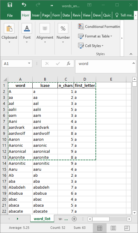
The code below shows how the data can be copied.

xlsclip <- read.table(file = "clipboard", sep = "\t", header = TRUE)

xlsclip %>%
    kable() %>%
    kable_styling(
        full_width = FALSE,
        position = "left"
    )

word	lcase	n_chars	first_letter
A	a	1	a
aa	aa	2	a
aal	aal	3	a
aalii	aalii	5	a
aam	aam	3	a
Aani	aani	4	a
aardvark	aardvark	8	a
aardwolf	aardwolf	8	a
Aaron	aaron	5	a
Aaronic	aaronic	7	a
Aaronical	aaronical	9	a
Aaronite	aaronite	8	a

9.12 Running system commands

R can run arbitrary system commands that you would normally run in a terminal or command window. The system() function is used to run commands, optionally with the results returned as a character vector. Under Mac and Linux, the usage is quite straightforward, for example, to list files in a specific directory:

tempdirfiles <- system("ls /tmp", intern = TRUE)

Under Windows, it takes a bit of extra code. To do the same requires the prefix cmd /c in the system() call before the command itself. Also any backslashes in path names need to be specified as double-backslashes for R.

# R prefers and automatically generates forward slashes
# under Windows, path delimiters are backslashes so need to be rendered in R as double backslashes
tmpdir <- dirname(tempdir()) %>% 
    str_replace_all("/", "\\\\")
# construct a system command
# under Windows 
cmd <- sprintf("cmd /c dir %s", tmpdir)
tempdirfiles <- system(command = cmd, intern = TRUE)

If you are running other programs or utilities that are executed in a terminal or command window, this can be very helpful.

9.13 Code styling

Good code should meet at least the two functional requirements of getting the job done and being able able to read. Code that gets the job done but that is not easy to read will cause problems later when you try to figure out how or why you did something.

The styler package can help clean up your code so that it conforms to a specific style such as that in the tidyverse style guide. styler can be integrated into RStudio for interactive use. It can reformat selected code, an entire file, or an entire project. An example is shown:

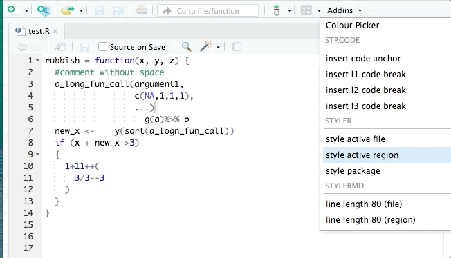
lintr is also useful for identifying potential style errors.

9.14 Session information

It may be helpful in troubleshooting or complete documentation to report the complete session information. For example, sometimes outdated versions of packages may contain errors. The session information is printed with sessionInfo().

sessionInfo()

## R version 4.0.4 (2021-02-15)
## Platform: x86_64-w64-mingw32/x64 (64-bit)
## Running under: Windows >= 8 x64 (build 9200)
## 
## Matrix products: default
## 
## locale:
## [1] LC_COLLATE=English_United States.1252  LC_CTYPE=English_United States.1252   
## [3] LC_MONETARY=English_United States.1252 LC_NUMERIC=C                          
## [5] LC_TIME=English_United States.1252    
## 
## attached base packages:
## [1] stats     graphics  grDevices utils     datasets  methods   base     
## 
## other attached packages:
##  [1] RVerbalExpressions_0.1.0 fst_0.9.4                lubridate_1.7.10         pdftools_2.3.1          
##  [5] captioner_2.2.3          animation_2.6            psych_2.0.12             pander_0.6.3            
##  [9] stargazer_5.2.2          readstata13_0.9.2        sf_0.9-7                 htmltools_0.5.1.1       
## [13] leaflet_2.0.4.1          tidycensus_0.11.4        sqldf_0.4-11             RSQLite_2.2.3           
## [17] gsubfn_0.7               proto_1.0.0              shiny_1.6.0              curl_4.3                
## [21] haven_2.3.1              kableExtra_1.3.4         knitr_1.31               magrittr_2.0.1          
## [25] forcats_0.5.1            stringr_1.4.0            dplyr_1.0.5              purrr_0.3.4             
## [29] readr_1.4.0              tidyr_1.1.3              tibble_3.1.0             ggplot2_3.3.3           
## [33] tidyverse_1.3.0         
## 
## loaded via a namespace (and not attached):
##   [1] readxl_1.3.1            uuid_0.1-4              backports_1.2.1         systemfonts_1.0.1      
##   [5] plyr_1.8.6              lazyeval_0.2.2          sp_1.4-5                crosstalk_1.1.1        
##   [9] digest_0.6.27           rsconnect_0.8.16        leaflet.providers_1.9.0 fansi_0.4.2            
##  [13] memoise_2.0.0           remotes_2.2.0           modelr_0.1.8            svglite_2.0.0          
##  [17] askpass_1.1             colorspace_2.0-0        blob_1.2.1              rvest_0.3.6            
##  [21] rappdirs_0.3.3          xfun_0.21               rgdal_1.5-23            tcltk_4.0.4            
##  [25] callr_3.5.1             crayon_1.4.1            jsonlite_1.7.2          tigris_1.0             
##  [29] glue_1.4.2              xmlparsedata_1.0.5      gtable_0.3.0            webshot_0.5.2          
##  [33] questionr_0.7.4         scales_1.1.1            qpdf_1.1                DBI_1.1.1              
##  [37] miniUI_0.1.1.1          Rcpp_1.0.6              viridisLite_0.3.0       xtable_1.8-4           
##  [41] tmvnsim_1.0-2           units_0.7-0             foreign_0.8-81          bit_4.0.4              
##  [45] DT_0.17                 htmlwidgets_1.5.3       rex_1.2.0               httr_1.4.2             
##  [49] RColorBrewer_1.1-2      ellipsis_0.3.1          pkgconfig_2.0.3         farver_2.1.0           
##  [53] sass_0.3.1              dbplyr_2.1.0            utf8_1.1.4              tidyselect_1.1.0       
##  [57] labeling_0.4.2          rlang_0.4.10            later_1.1.0.1           munsell_0.5.0          
##  [61] cellranger_1.1.0        tools_4.0.4             cachem_1.0.4            cli_2.3.1              
##  [65] generics_0.1.0          broom_0.7.5             evaluate_0.14           fastmap_1.1.0          
##  [69] yaml_2.2.1              rematch2_2.1.2          processx_3.4.5          bit64_4.0.5            
##  [73] fs_1.5.0                nlme_3.1-152            mime_0.10               xml2_1.3.2             
##  [77] compiler_4.0.4          rstudioapi_0.13         png_0.1-7               e1071_1.7-4            
##  [81] reprex_1.0.0            bslib_0.2.4             stringi_1.5.3           cyclocomp_1.1.0        
##  [85] highr_0.8               ps_1.6.0                desc_1.2.0              lattice_0.20-41        
##  [89] classInt_0.4-3          styler_1.3.2            vctrs_0.3.6             pillar_1.5.1           
##  [93] lifecycle_1.0.0         jquerylib_0.1.3         data.table_1.14.0       maptools_1.0-2         
##  [97] httpuv_1.5.5            Rmisc_1.5               R6_2.5.0                bookdown_0.21          
## [101] promises_1.2.0.1        KernSmooth_2.23-18      codetools_0.2-18        assertthat_0.2.1       
## [105] chron_2.3-56            rprojroot_2.0.2         withr_2.4.1             mnormt_2.0.2           
## [109] parallel_4.0.4          hms_1.0.0               lintr_2.0.1             grid_4.0.4             
## [113] labelled_2.7.0          class_7.3-18            rmarkdown_2.7

9.15 Comment out Rmd/HTML code

To comment out entire parts of your Rmd so they do not appear in your rendered HTML, use HTML comments, which are specified with the delimiters <!-- and -->.

9.16 Source code

09-week09.Rmd

cat(readLines(con = "09-week09.Rmd"), sep = "\n")

# Week 9 {#week9}

```{r, echo=FALSE, warning=FALSE, message=FALSE}
library(tidyverse)
library(magrittr)
library(knitr)
library(kableExtra)
library(haven)
library(curl)
library(ggplot2)
```

<h2>Topic: Miscellaneous data processing </h2>
This week's lesson will cover a set of miscellaneous data processing topics.

Mostly this is a set of coded examples with explanations

## Substituting text

### `paste()`, `paste0()`

Pasting text allows you to substitute variables within a text string. For example, if you are running a long loop over a series of files and you want to know which file name and loop iteration you are on. 

The function `paste()` combines a set of strings and adds a space between the strings, e.g., combining the first values from the `LETTERS` and the `letters` built-in vectors:

```{r}
paste(LETTERS[1], letters[1])
```

whereas `paste0` does not add spaces:

```{r}
paste0(LETTERS[1], letters[1])
```

Download the file [quickfox](files/quickfox.zip) to an arbitrary location on your computer. The code below assumes it was stored in `r dirname(tempdir())`.

```{r}
# a temp location--get dirname of dirname of the tempdir
tmp <- tempdir() %>%
    dirname()
# zip file
zipfile <- file.path(tmp, "quickfox.zip")
# unzip
unzip(zipfile = zipfile, overwrite = TRUE, exdir = tmp)
# files in the zipfile
fnames <- unzip(zipfile = file.path(tmp, "quickfox.zip"), list = TRUE) %>%
    pull(Name) %>%
    file.path(tmp, .)

# read each file
for (i in seq_len(length(fnames))) {
    # the file name
    fname <- fnames[i]
    # read the file
    mytext <- scan(file = fname, what = "character", quiet = TRUE)

    # vvvvvvvvvvvvvvvvvvvvvvvvvvvvvv
    # make a string using `paste()`
    mystr <- paste(mytext, "    ", i, "of", length(fnames), fname)
    # ^^^^^^^^^^^^^^^^^^^^^^^^^^^^^^

    # print the message
    message(mystr)
}
```


### `sprintf()`
`sprintf()` can be used to format text. Here are just a few examples. The result is a formatted text string.

#### Formatting numerical values
<u>Leading zeros</u>

Numeric values can be formatted with a specific number of decimal places or leading zeros. For example, ZIP codes imported from CSV files often are converted to integers. The following code chunk converts some numerical ZIP code-like values to text values with the correct format.

Bad ZIP codes:
```{r}
# some numerical ZIP codes
(zip_bad <- data.frame(id = 1:3, zipcode = c(90201, 02134, 00501)))
```

Good ZIP codes:
```{r}
# fix them up
(zip_good <- zip_bad %>% mutate(
    zipcode = sprintf("%05d", zipcode)
))
```

<u>Decimal places</u>

Numerical values with different numbers of decimal places can be rendered with a specific number of decimal places. 

```{r}
# numers with a variety of decimal places
v <- c(1.2, 2.345, 1e+5 + 00005)

# four fixed decimal places
v %>% sprintf("%0.4f", .)
```

Note that this is distinct from `round()`, which results in a numeric vector:

```{r}
# round to 4 places
v %>% round(., 4)
```

#### String substitutions
`sprintf()` can also be used to achieve the same substitution in the file reading loop above. Each `%s` is substituted in order of the position of the arguments following the string. Also note that `\t` inserts a `TAB` character.

```{r}
# read each file
for (i in seq_len(length(fnames))) {
    # the file name
    fname <- fnames[i]
    # read the file
    mytext <- scan(file = fname, what = "character", quiet = TRUE)

    # vvvvvvvvvvvvvvvvvvvvvvvvvvvvvv
    # make a string using `paste()`
    mystr <- sprintf("%s\t%s of %s:\t%s", mytext, i, length(fnames), fname)
    # ^^^^^^^^^^^^^^^^^^^^^^^^^^^^^^

    # print the message
    cat(mystr)
}
```

### `str_replace()`, `str_replace_all()`
The `stringr` functions `str_replace()` and `str_replace_all()` can be used to substitute specific strings in other strings. For example, we might create a generic function to run over a set of subject IDs that generates a file for each subject.

```{r}
subjects <- c("a1", "b2", "c3")

f <- function(id) {
    # create an output filename by substituting in the subject ID
    outfname <- "C:/temp/xIDx.csv" %>% str_replace(pattern = "xIDx", id)
    # ... do a bunch of stuff, for example
    val <- rnorm(1)
    # write the file
    message(paste0("writing"))
    write.csv(x = val, file = outfname)
}

for (i in subjects) {
    f(i)
}
```

## Showing progress
A text-based progress bar can be shown using `txtProgressBar()`. Here we run the same loop for reading the text files, but rather than printing the loop iteration and file names, we show the progress bar and the file contents. If no text is printed to the console (unlike what is demonstrated below with `cat()`), the progress bar will not print on several lines.

```{r}
n_fnames <- length(fnames)
# create progress bar
pb <- txtProgressBar(min = 0, max = n_fnames, style = 3)
for (i in 1:n_fnames) {
    # delay a bit
    Sys.sleep(0.1)
    # update progress bar
    setTxtProgressBar(pb, i)
    # read and print from the file
    txt <- scan(fnames[i], what = "character", quiet = TRUE)
    cat("\n", txt, "\n")
}
close(pb)
```

## Turning text into code: `eval(parse(text = "some string"))`
Sometimes you may have variables whose values that you want to use in a command or function. For example, suppose you wanted to write a set of files, one for each ZIP code in a data frame, with a file name including the ZIP code. We would not want to use the column name `zipcode`, but we want the actual value. 

We can generate a command using some kind of text substitution as above with `sprintf()`

```{r}
for (i in zip_good %>% pull(zipcode)) {
    # do some stuff
    vals <- rnorm(n = 3)
    y <- bind_cols(zipcode = i, v = vals)
    # a writing command using sprintf() to substitute %s = ZIP code
    cmd <- sprintf("write.csv(x = y, file = 'C:/temp/%s.csv', row.names = FALSE)", i)

    # this runs the command
    eval(parse(text = cmd))
}
```

## SQL in R with `RSQLite` and `sqldf`
Sometimes R's syntax for processing data can be difficult and confusing. For programmers who are familiar with structured query language (SQL), it is possible to run SQL statements within R using a supported database back end (by default SQLite) and the `sqldf()` function.

For example, the mean sepal length by species from the built-in `iris` data set can be obtained, presented in Table \@ref(tab:iris)

```{r iris}
library(sqldf)

sqlc <- 'select 
    "Species" as species
    , avg("Sepal.Length") as mean_sepal_length
from iris
group by "Species";
'

iris_summary <- sqldf(x = sqlc)

iris_summary %>% 
    kable(caption = "Mean sepal length from the iris data set") %>% 
    kable_styling(full_width = FALSE, position = "left")
```




## Downloading files from password-protected web sites
Some web sites are protected by simple username/password protection. For example, try opening [http://staff.washington.edu/phurvitz/csde502_winter_2021/password_protected] (http://staff.washington.edu/phurvitz/csde502_winter_2021/password_protected). The username/password pair is csde/502, which will allow you to see the contents of the web folder.

If you try downloading the file through R, you will get an error because no password is supplied.

```{r}
try(
    read.csv("http://staff.washington.edu/phurvitz/csde502_winter_2021/password_protected/foo.csv")
)
```

However, the username and password can be supplied as part of the URL, as below. When the username and password are supplied, they will be cached for that site for the duration of the R session.

```{r}
try(
    read.csv("http://csde:502@staff.washington.edu/phurvitz/csde502_winter_2021/password_protected/foo.csv")
)
```


## Dates and time stamps: `POSIXct` and `lubridate`
R uses POSIX-style time stamps, which are stored internally as the number of fractional seconds from January 1, 1970. It is imperative that the control over time stamps is commensurate with the temporal accuracy and precision  your data. For example, in the measurement of years of residence, precision is not substantially important. For measurement of chemical reactions, fractional seconds may be very important. For applications such as merging body-worn sensor data from GPS units and accelerometers for estimating where and when physical activity occurs, minutes of error can result in statistically significant mis-estimations.

For example, you can see the numeric value of these seconds as `options(digits = 22); Sys.time() %>% as.numeric()`.

```{r}
options(digits = 22)
Sys.time() %>% as.numeric()
```

If you have time stamps in text format, they can be converted to POSIX time stamps, e.g., the supposed time Neil Armstrong stepped on the moon:

```{r}
(eagle <- as.POSIXct(x = "7/20/69 10:56 PM", tz = "CST6CDT", format = "%m/%d/%y %H:%M"))
```

Formats can be specified using specific codes, see `strptime()`.

The `lubridate` package has a large number of functions for handling date and time stamps. For example, if you want to convert a time stamp in the current time zone to a different time zone, first we get the current time

```{r}
library(lubridate)
# set the option for fractional seconds
options(digits.secs = 3)
(now <- Sys.time() %>% strptime("%Y-%m-%d %H:%M:%OS"))
```

And convert to UTC:

```{r}
# show this at time zone UTC
(with_tz(time = now, tzone = "UTC"))
```

or show in a different format:

```{r}
# in different format
now %>% format("%A, %B %d, %Y %l:%m %p %Z")
```

```{r, echo=FALSE}
# reset the digits
options(digits = 7)
```

## Timing with `Sys.time()` and `difftime()`
It is easy to determine how long a process takes by using sequential `Sys.time()` calls, one before and one after the process, and getting the difference with `difftime()`. For example, 

```{r}
# mark time and run a process
t0 <- Sys.time()
Sys.sleep(5)
t1 <- Sys.time()

# difftime() unqualified will make its best decision about what to print
(difftime(time1 = t1, time2 = t0))

# time between moon step and now-ish
(difftime(time1 = t0, time2 = eagle))
```

`difftime()` can also be forced to report the time difference in the units of choice:

```{r}
(difftime(time1 = t1, time2 = t0, units = "secs") %>% as.numeric()) %>% round(0)
(difftime(time1 = t1, time2 = t0, units = "mins") %>% as.numeric()) %>% round(2)
(difftime(time1 = t1, time2 = t0, units = "hours") %>% as.numeric()) %>% round(4)
(difftime(time1 = t1, time2 = t0, units = "days") %>% as.numeric()) %>% round(6)
```

## Faster files with `fst()`
The `fst` package is great for rapid reading and writing of data frames. The format can also result in much smaller file sizes using compression. Here we will examine the large Add Health file. First, a download, unzip, and read as necessary:

```{r}
library(fst)
myUrl <- "http://staff.washington.edu/phurvitz/csde502_winter_2021/data/21600-0001-Data.dta.zip"
# zipfile in $temp
tmp <- tempdir() %>% dirname()
zipfile <- file.path(tmp, basename(myUrl))
# dta file in $temp
dtafname <- tools::file_path_sans_ext(zipfile)
# check if the dta file exists
if (!file.exists(dtafname)) {
    # if the dta file doesn't exist, check for the zip file
    # check if the zip file exists, download if necessary
    if (!file.exists(zipfile)) {
        curl::curl_download(url = myUrl, destfile = zipfile)
    }
    # unzip the downloaded zip file
    unzip(zipfile = zipfile, exdir = Sys.getenv("TEMP"))
}

# read the file
dat <- read_dta(dtafname)

# save as a CSV, along with timing
t0 <- Sys.time()
csvfname <- dtafname %>% str_replace(pattern = "dta", replacement = "csv")
write.csv(x = dat, file = csvfname, row.names = FALSE)
t1 <- Sys.time()
csvwrite_time <- difftime(time1 = t1, time2 = t0, units = "secs") %>%
    as.numeric() %>%
    round(1)

# file size
csvsize <- file.info(csvfname) %>% pull(size) %>% sprintf("%0.f", .)

# save as FST, along with timing
t0 <- Sys.time()
fstfname <- dtafname %>% str_replace(pattern = "dta", replacement = "fst")
write.fst(x = dat, path = fstfname)
t1 <- Sys.time()

# file size
fstsize <- file.info(fstfname) %>% pull(size) %>% sprintf("%0.f", .)
fstwrite_time <- difftime(time1 = t1, time2 = t0, units = "secs") %>%
    as.numeric() %>%
    round(1)
```

It took `r csvwrite_time` s to write `r csvsize` bytes as CSV, and `r fstwrite_time` s to write `r fstsize` bytes as a FST file (with the default compression amount of 50). Reading speeds are comparable.

___It should be noted___ that some file attributes will not be saved in FST format and therefore it should be used with caution if you have a highly attributed data set (e.g., a Stata DTA file with extensive labeling). You will lose those attributes! But for data sets with a simple structure, including factors, the FST format is a good option.

## Getting US Census data with `tigris`, `tidycensus`
Dealing with US Census data can be overwhelming, particularly if using the raw text-based data. The Census Bureau has an API that allows more streamlined downloads of variables (as data frames) and geographies (as simple format shapes). It is necessary to get an API key, available for free. See [tidycensus](https://walker-data.com/tidycensus/) and  [tidycensus basic usage](https://walker-data.com/tidycensus/articles/basic-usage.html).

`tidycensus` uses [`tigris`](https://www.rdocumentation.org/packages/tigris/versions/1.0), which downloads the geographic data portion of the census files.

A simple example will download the variables representing the count of White, Black/African American, American Indian/Native American, and Asian persons from the American Community Survey (ACS) data for King County in 2019. 

The labels from the census API are:

```
"Estimate!!Total"                                         
"Estimate!!Total!!White alone"                            
"Estimate!!Total!!Black or African American alone"        
"Estimate!!Total!!American Indian and Alaska Native alone"
"Estimate!!Total!!Asian alone" 
```

```{r, warning=FALSE}
library(tidycensus)
# the census variables
census_vars <- c(
    p_denom_race = "B02001_001",
    p_n_white = "B02001_002",
    p_n_afram = "B02001_003",
    p_n_aian = "B02001_004",
    p_n_asian = "B02001_005"
)

# get the data
ctdat <- get_acs(
    geography = "tract",
    variables = census_vars, 
    cache_table = TRUE, 
    year = 2019, 
    output = "wide", 
    state = "WA", 
    county = "King", 
    geometry = TRUE,
    survey = "acs5"
)
```

A few values are shown in Table \@ref(tab:census), and a simple map is shown in \@ref(fig:ct), with percent African American residents and tract identifier.

```{r census}
# print a few records
ctdat %>%
    head() %>%
    kable(caption = "Selected census tract variables from the 5-year ACS from 2019 for King County, WA") %>%
    kable_styling(full_width = FALSE, position = "left")
```

```{r, fig.cap="Percent African American in census tracts in King County, 2019 ACS 5-year estimate", warning=FALSE, message=FALSE}
library(leaflet)
library(htmltools)
library(sf)

# define the CRS
st_crs(ctdat) <- 4326

# proportion Black
ctdat %<>% 
    mutate(pct_black = (p_n_aframE / p_denom_raceE * 100) %>% round(1))

# a label
labels <- sprintf("%s<br/>%s%s", ctdat$GEOID, ctdat$pct_black, "%") %>% lapply(htmltools::HTML)

bins <- 0:50
pal <- colorBin(palette = "Reds", 
                domain = ctdat$pct_black, 
                bins = bins)

bins2 <- seq(0, 50, by = 10)
pal2 <- colorBin(palette = "Reds", 
                domain = ctdat$pct_black, 
                bins = bins2)

# the leaflet map
m <- leaflet(height = "500px") %>% 
    # add polygons from tracts
    addPolygons(
        data = ctdat, 
        weight = 1, 
        fillOpacity = 0.8,
        # fill using the palette
        fillColor = ~pal(pct_black),
        # highlighting
        highlight = highlightOptions(
            weight = 5,
            color = "#666",
            fillOpacity = 0.7,
            bringToFront = TRUE),
        # popup labels
        label = labels,
        labelOptions = labelOptions(
            style = list("font-weight" = "normal", padding = "3px 8px"),
            textsize = "15px",
            direction = "auto")) %>% 
    addLegend(position = "bottomright", pal = pal2, values = ctdat$pct_black,
          title = "% African American",
          opacity = 1)
m %>% addTiles()
```


## Easier regular expressions with `RVerbalExpressions`
Regular expressions are powerful but take some time and trial-and-error to master. The `RVerbalExpresions` package can be used to more easily generate regular expressions. See the help for `rx()` and associated functions.

These examples show two constructions of regular expressions for matching two similar but different URLs.

```{r}
library(RVerbalExpressions)
# a pattern
x <- rx_start_of_line() %>%
    rx_find("http") %>%
    rx_maybe("s") %>%
    rx_find("://") %>%
    rx_maybe("www.") %>%
    rx_anything_but(" ") %>%
    rx_end_of_line()

# print the expression
(x)

# search for a pattern in some URLs
urls <- c(
    "http://www.google.com",
    "http://staff.washington.edu/phurvitz/csde502_winter_2021/"
)
grepl(pattern = x, x = urls)


# a different pattern
y <- rx_start_of_line() %>%
    rx_find("http") %>%
    rx_maybe("s") %>%
    rx_find("://") %>%
    rx_find("www.") %>%
    rx_anything_but(" ") %>%
    rx_end_of_line()

# print the expression
(y)

# search for a pattern in the two URLs, matches one, does not match the other
grepl(pattern = y, x = urls)
```

## Quick copy from Excel (Windows only)
Under Windows, it is possible to copy selected cells from an Excel worksheet directly to R. This is not an endorsement for using Excel, but there are some cases in which Excel may be able to produce some quick data that you don't want to develop in other ways.

As a demonstration, you can use [analysis.xlsx](files/words_analysis.xlsx). Download and open the file. Here is shown a selection of cells that was copied. 

![](images/week09/excel.png)

The code below shows how the data can be copied.

```{r, echo=FALSE}
xlsclip <- fst::read.fst("files/xlsclip.fst")
```

```{r, eval=FALSE}
xlsclip <- read.table(file = "clipboard", sep = "\t", header = TRUE)

xlsclip %>%
    kable() %>%
    kable_styling(
        full_width = FALSE,
        position = "left"
    )
```

```{r, echo=FALSE}
xlsclip %>%
    kable() %>%
    kable_styling(
        full_width = FALSE,
        position = "left"
    )
```

## Running system commands
R can run arbitrary system commands that you would normally run in a terminal or command window. The `system()` function is used to run commands, optionally with the results returned as a character vector. Under Mac and Linux, the usage is quite straightforward, for example, to list files in a specific directory:

```
tempdirfiles <- system("ls /tmp", intern = TRUE)
```

Under Windows, it takes a bit of extra code. To do the same requires the prefix `cmd /c` in the `system()` call before the command itself. Also any backslashes in path names need to be specified as double-backslashes for R.

```{r}
# R prefers and automatically generates forward slashes
# under Windows, path delimiters are backslashes so need to be rendered in R as double backslashes
tmpdir <- dirname(tempdir()) %>% 
    str_replace_all("/", "\\\\")
# construct a system command
# under Windows 
cmd <- sprintf("cmd /c dir %s", tmpdir)
tempdirfiles <- system(command = cmd, intern = TRUE)
```

If you are running other programs or utilities that are executed in a terminal or command window, this can be very helpful.

## Code styling
Good code should meet at least the two functional requirements of getting the job done and being able able to read. Code that gets the job done but that is not easy to read will cause problems later when you try to figure out how or why you did something.

The [`styler`](https://github.com/r-lib/styler) package can help clean up your code so that it conforms to a specific style such as that in the [tidyverse style guide](https://style.tidyverse.org/). `styler` can be integrated into RStudio for interactive use. It can reformat selected code, an entire file, or an entire project. An example is shown:

![](images/week09/styler_0.1.gif)

[`lintr`](https://github.com/jimhester/lintr) is also useful for identifying potential style errors.

## Session information
It may be helpful in troubleshooting or complete documentation to report the complete session information. For example, sometimes outdated versions of packages may contain errors. The session information is printed with `sessionInfo()`.

```{r}
sessionInfo()
```

## Comment out Rmd/HTML code
To comment out entire parts of your Rmd so they do not appear in your rendered HTML, use HTML comments, which are specified with the delimiters `<!--` and `-->`.

## Source code
[09-week09.Rmd](09-week09.Rmd)
```{r comment=''}
cat(readLines(con = "09-week09.Rmd"), sep = "\n")
```