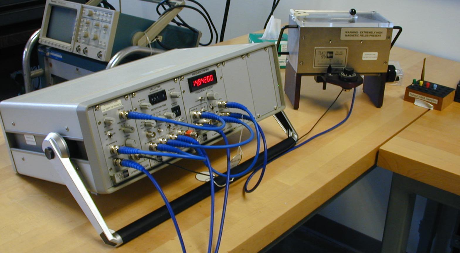
TeachSpin PS1 Pulsed NMR Spectrometer
Bloch.py
Hahn.py
NMR Simulations and Videos
NMR and The Bloch Equation
Nuclear magnetic resonance (NMR) is well modeled by the Bloch equation:
\begin{equation} \label{eq:Bloch} \frac{d\bvec{M}}{dt} = -\gamma\bvec{H}\times\bvec{M} - \frac{\bvec{M}-\chi\bvec{H}}{T} \;, \end{equation}
in which $\bvec{M}$ is the net magnetization of the material subject to applied field $\bvec{H}$, $\gamma$ is the gyromagnetic ratio of the nuclei that contribute to $\bvec{M}$, $\chi$ is the magnetic susceptibility of the material (typically taken to follow a Curie law) and $T$ is a relaxation time constant, equal to $T_1$ for the z-component (parallel to $\bvec{H}_0$) or $T_2$ for the x,y-components. The central resonance frequency $\omega_0=\gamma H_0$.
The evolution of magnetization $\bvec{M}$, under an alternating field used to induce resonance, is complicated. In a static field, $\bvec{M}$ executes a simple precession about $\bvec{H}$, but with the RF turned on, $\bvec{M}$ may follow a spiral that inverts it relative to $\bvec{H}_0$ if the RF frequency matches the resonance, or a partial spiral if off-resonance. At the same time, $\bvec{M}$ evolves toward a steady state according to the time constants $T_1$ and $T_2$.
Although the Bloch equation models the overall magnetization well, it alone cannot yield the fascinating phenomenon of spin echoes. These occur because of variations across the sample in the local static field: each tiny region of the sample has its own resonance frequency. Under fairly common conditions, following a brief RF pulse, each region evolves according to its own coherence, but the initial signal disappears because of loss of phase alignment from region to region. By applying subsequent RF pulses, one sees "echoes," which signal the rephasing of the regions that initially dephased. The theory requires an ensemble calculation, with each member evolving by its own copy of the Bloch equation. The signal is found by calculating the ensemble average.
The Simulations
Understanding the origin of NMR signals, and the behavior of the Bloch equation in single and in ensemble contexts, is greatly aided through animated simulations.
The simulations presented here were written with VPython, and are made available through the service Web VPython (a.k.a. Glowscript).
VPython was developed by David Scherer, Bruce Sherwood and others, and is currently maintained by Bruce Sherwood. It is ideally suited for rapid development of 3D physics-based animations. The browser-based Web VPython leverages Python to create smooth animations by “transpiling” Python into JavaScript which is optimized for browsers. (Google Chrome and similar are recommended.) Plus, the scripts are easily shareable via URLs (see below).
The animations simulate dynamics of the Bloch equation and its extension into ensemble evolution. They reveal aspects of spin dynamics that are hard to imagine, such as internal symmetries and unexpected limiting configurations, and provide welcome clarity to complex NMR phenomena such as pulse-width errors and non-resonance conditions.
The Bloch Equation Simulation
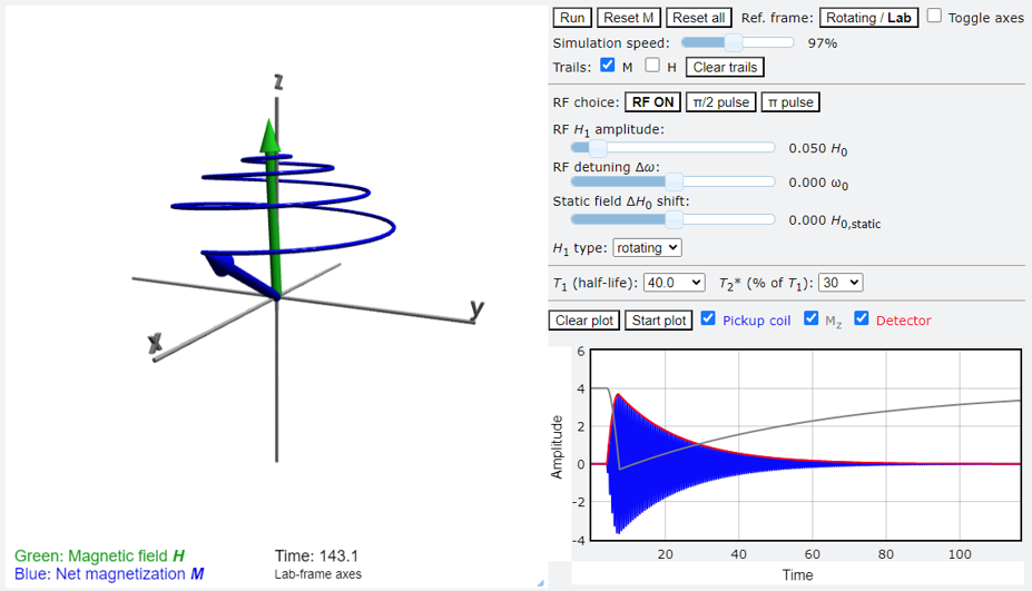
The Python program Bloch.py illustrates the basic evolution of a single magnetization $\bvec{M}$ under the influence of an applied magnetic field $\bvec{H}$, plus relaxation according to time constants $T_1$ and $T_2^*$. The user can adjust all parameters of the applied field, and select from a range of time constants.
A focus of the simulation is to show the transformation of coordinate systems from the "lab" to the "rotating" frame. The coordinate axes may be switched between the frames independently of the frame itself.
This simulation does not produce spin echoes, as there is only one magnetization But it can simulate the inversion-sequence measurement of $T_1$, as well as free induction decay (FID).
The Ensemble Simulation and Spin Echoes
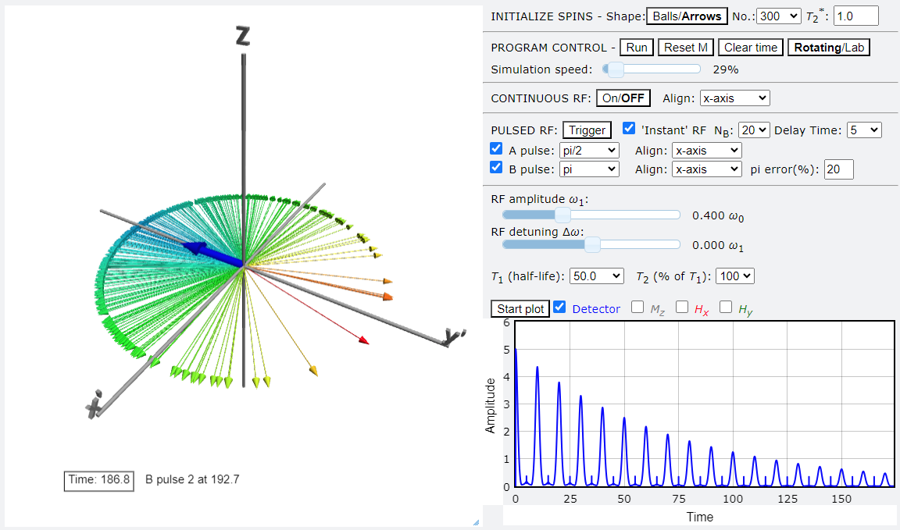
Hahn.py extends Bloch.py in two ways: (1) It creates an ensemble of "isochromes" (in Hahn's terminology) $\{\bvec{M}_i\}$ where each member evolves according to the Bloch equation with its own resonance frequency $\omega_i$ which are distributed normally about the central resonance at $\omega_0$; (2) the effect of the applied RF can be programmed to be on for predetermined amounts, sufficient to cause a fixed rotation, for example, a $\pi/2$ pulse. Also, the simulation runs mainly in the rotating frame, which is where most NMR physics is done.
By means of the ensemble, the relaxation time constants can be fully separated into $T_1$ and $T_2$, with $T_2^*$ now a consequence of the spread of resonances within the ensemble. This allows a complete simulation of spin echoes, as they are clearly seen to be a consequence of preserved coherence within the ensemble.
Some Lessons with the Simulations
LESSON 1 – The Rotating Reference Frame
It is straightforward to prove that the Bloch equation looks the same in a reference frame that rotates with an applied rotating field $\bvec{H}_1(t) = H_1\left(\ihat\cos\omega t - \jhat\sin\omega t\right)$. By this, the complicated motion of $\bvec{M}$ is shown as a sum of two simpler ones. We define the basis of the rotating frame with
\begin{align} \label{eq:prime_basis} \ihat^{\prime} & = \ihat\cos\omega t - \jhat\sin\omega t\\ \jhat^{\prime} & = \ihat\sin\omega t + \jhat\cos\omega t\nonumber\;. \end{align}In this reference frame, the net magnetic field then becomes constant:
\begin{equation}\label{eq:H_eff} \bvec{H}_\text{eff} = H_1\ihat^{\prime} + \left(H_0 - \frac{\omega}{\gamma}\right)\khat\;. \end{equation}Then the motion of $\bvec{M}$ is a simple precession about $\bvec{H}_\text{eff}$. On resonance $\omega=\omega_0=\gamma H_0$ and precession is about $\ihat^{\prime}$ only. What does the reference frame shift look like? The simulation allows one to observe the transformation directly:
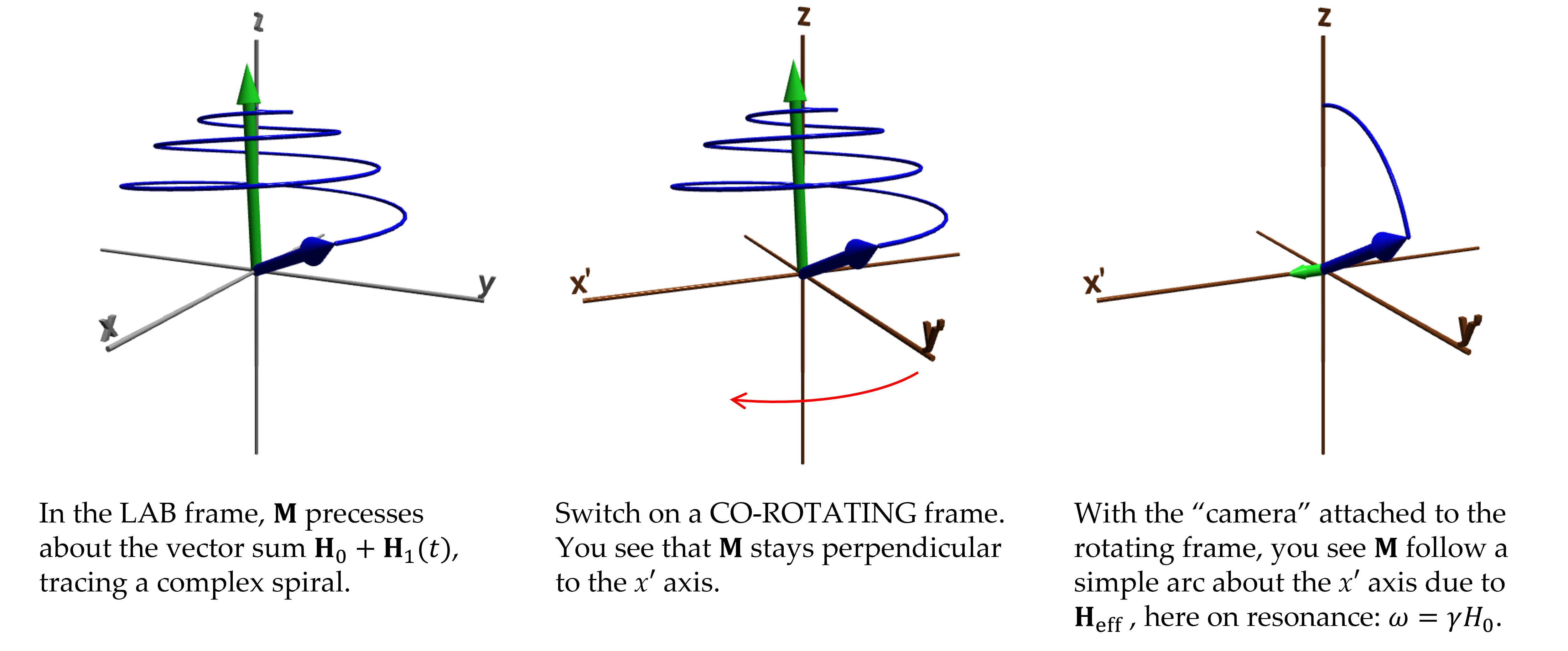
We see that in the rotating reference frame, on resonance, the constant field in the z direction $\bvec{H}_0$ vanishes, leaving only the applied RF, which is now appears as a steady field along the x$^{\prime}$ axis.
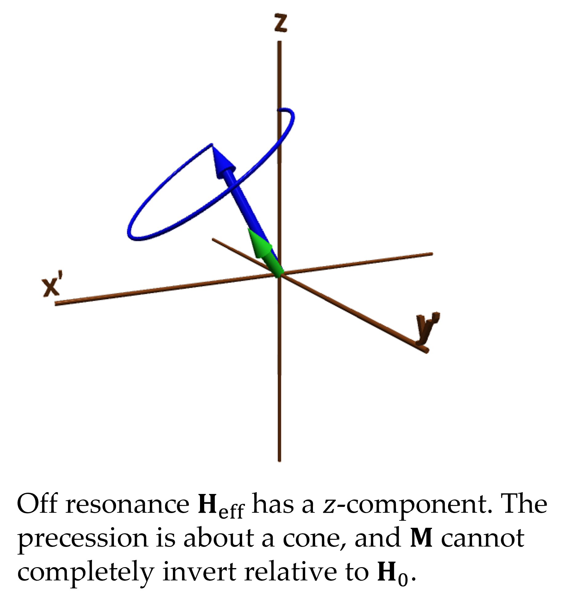
Off-Resonance
Simply by changing the frequency of the RF, in the rotating frame of reference one sees the direction of the effective field change. If the RF is tuned below resonance, the effective field tilts up, if it is tuned above resonance, it tilts down. An upward tilt causes a component of the precession to be in the same direction as the original steady field $\bvec{H}_0$. A downward tilt causes precession opposite, indicating that the rotating frame is faster than the resonance frequency.
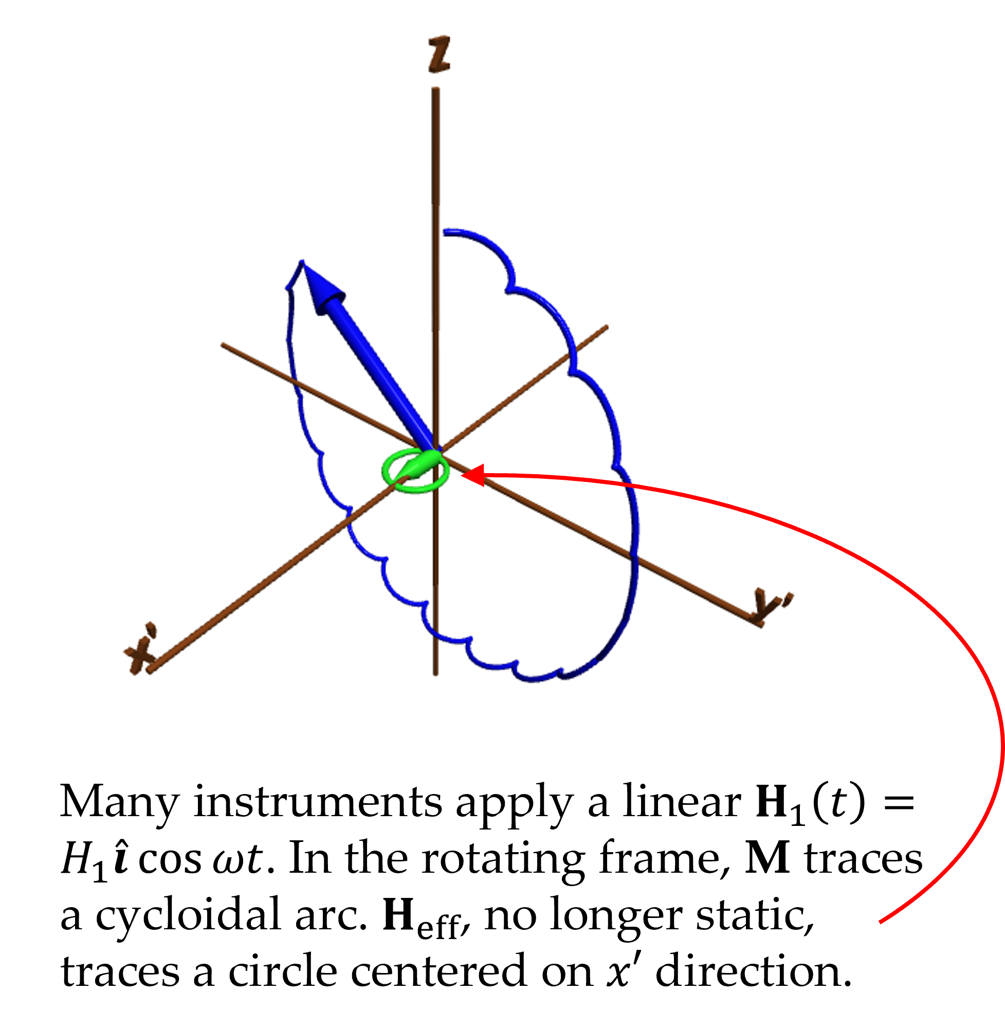
Linearly Oscillating Field
A linearly oscillating RF field $\bvec{H}_1(t)=2H_1\ihat\cos\omega t$ can be decomposed into two counter-rotating fields: one that rotates with the rotating frame, and is therefore constant in that frame, and another that rotates against the rotating frame, and is therefore rotating at twice its frequency in that frame. The combined field in the rotating frame is thus circular at twice the frequency, but offset in the direction of the steady field. This is seen as a field that grows and shrinks mainly in one direction, and $\bvec{M}$ follows the same general arc as with the purely rotating field, but its path is modulated by a cycloidal oscillation.
LESSON 2 - T1, T2, and T2*
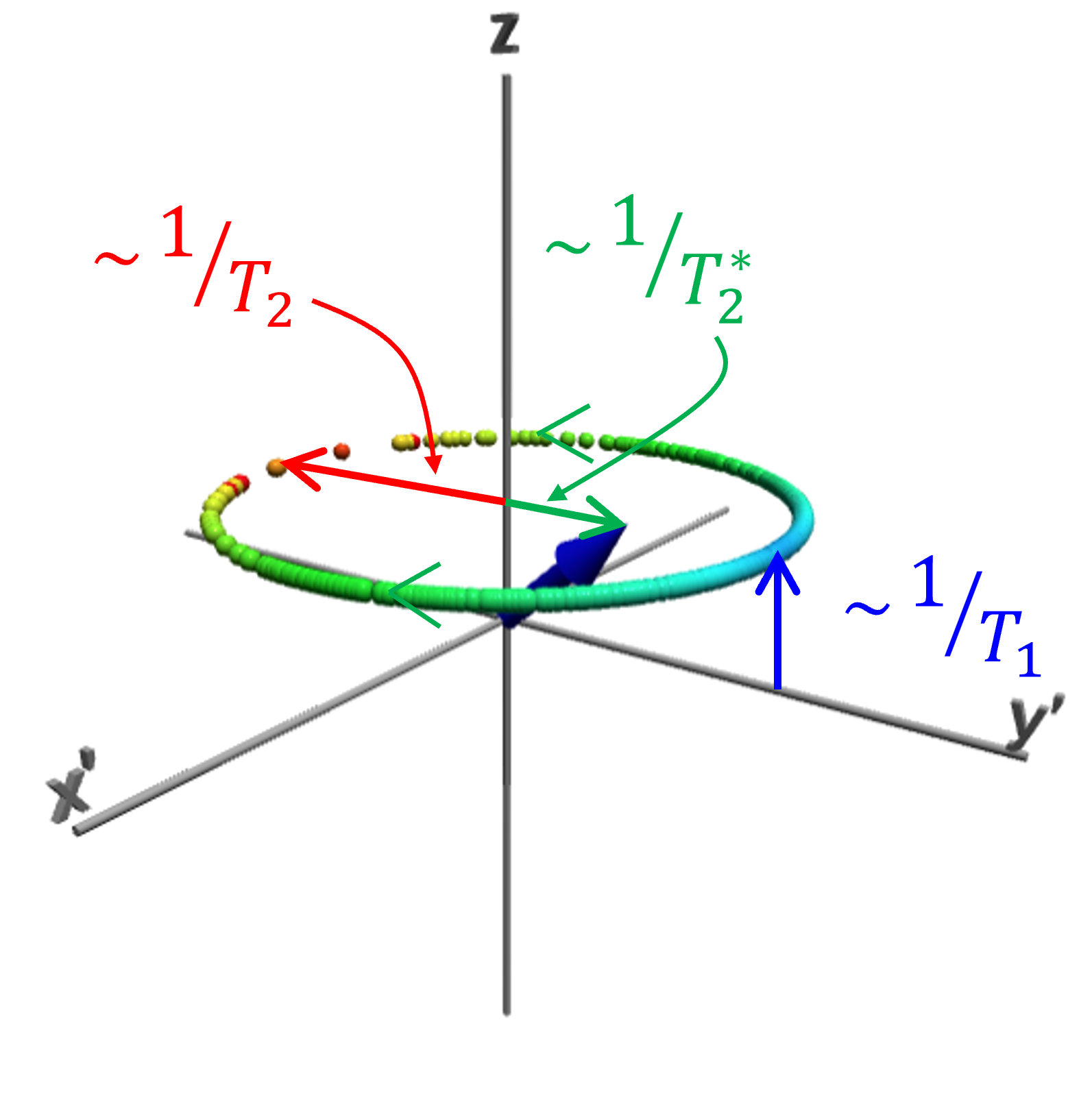
In the Bloch equation, $T_1$ and $T_2$ represent relaxation processes. But, after $\bvec{H}_1$ is removed, the "free induction" signal decays according to $T_2^*$ which depends on the instrument: precession speeds within the sample vary according to the local value of $H_0$. The simulation creates an ensemble of magnetizations, i.e., "isochromes" (Hahn’s term) $\{\bvec{M}_i\}$, each with its own resonant frequency $\omega_{0,i}=\omega_0+\Delta\omega_i$, with $\{\Delta\omega_i\}$ normally distributed. Each member of the ensemble is represented by a point (or arrow) with the position of the point at $\bvec{M}_i$. The net magnetization $\bvec{M}$ is the average of the ensemble.
All $\bvec{M}_i$ evolve according to the same values of $T_1$ and $T_2$. $T_2^*$ sets isochrome dephasing, seen as the points dispersing about the z-axis. Following a $\pi/2$ pulse, $\{\bvec{M}_i\}$ disperse into a circle. The radius of the circle decreases according to $T_2$, the center of the circle evolves along the z axis toward equilibrium according to $T_1$, and the radial component of $\bvec{M}$ depends mostly on $T_2^*$ when $T_2^*\ll T_2$.
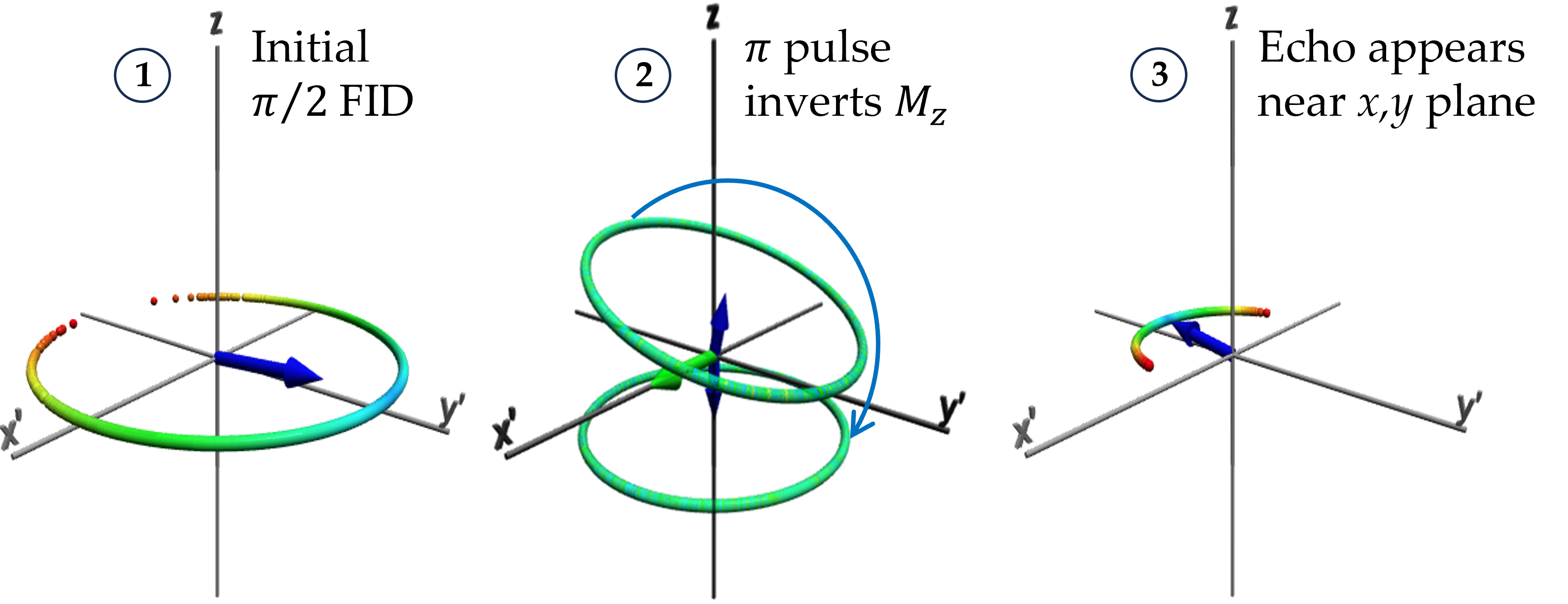
LESSON 3 – Hahn’s Spin Echoes
Erwin Hahn, who discovered and explained spin echoes in 1950, thought, at first, the signal at time $t=2\tau$ that he saw following two "$\pi/2$" pulses (the first at $t=0$ and the second at $t=\tau$, here $\tau=5$ time units) was an artifact of his electronics. In fact, it was evidence that the isochromes dispersed in phase following the first pulse were refocused by the second pulse. The strongest echo results from a second pulse that inverts the ensemble completely: a "$\pi$" pulse. But spin echoes appear after almost any type of second pulse. This lesson shows the ensemble configuration deduced by Hahn and Purcell from two $\pi/2$ pulses, what Hahn named the "eight ball."
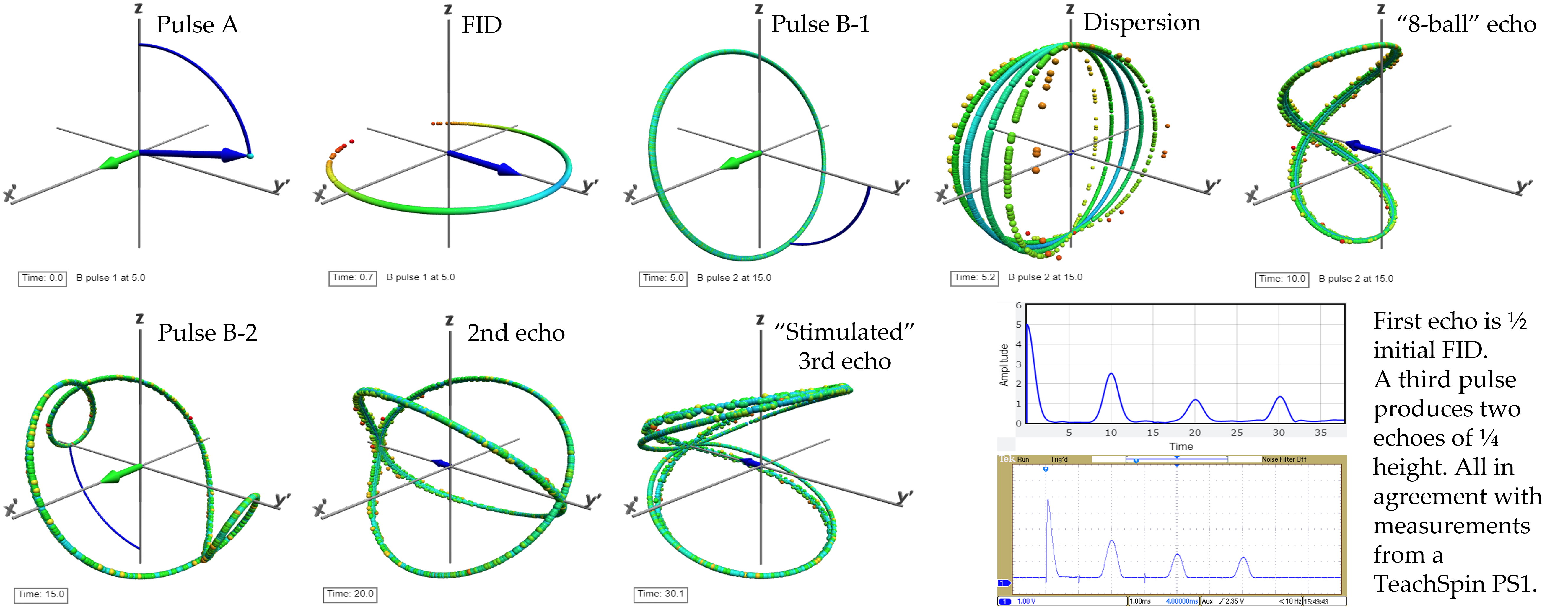
As shown above, a third $\pi/2$ pulse applied at $t=3\tau$ generates two more echoes. The first is stimulated by the echo at $2\tau$ and appears at $t=4\tau$. The second is stimulated by the initial free induction decay at $t=0$ and appears at $t=6\tau$ or $2\times3\tau$.
LESSON 4 – Multipulse Sequences
The pulsed NMR method extracts information about the sample usually through multipulse sequences. The ensemble simulation shows how signals arise through the complex evolution of the ensemble members. Here are three examples.
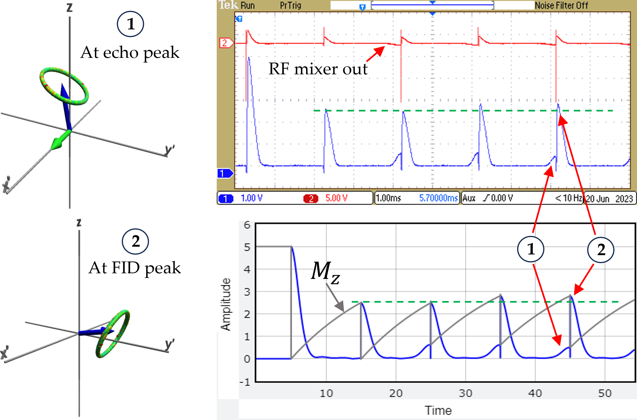
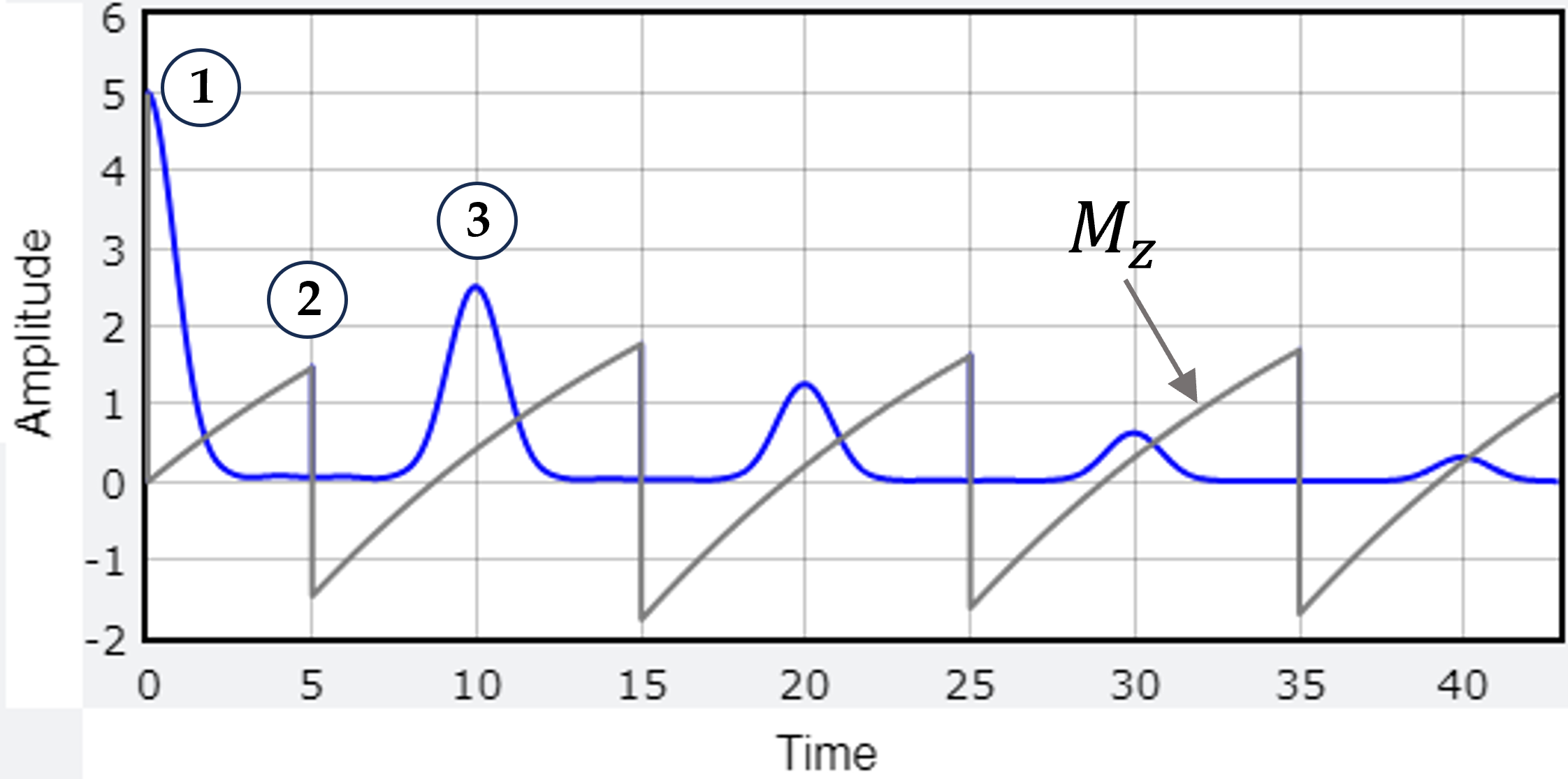
A. T1 Measurement from π/2 Pulse Repetition.
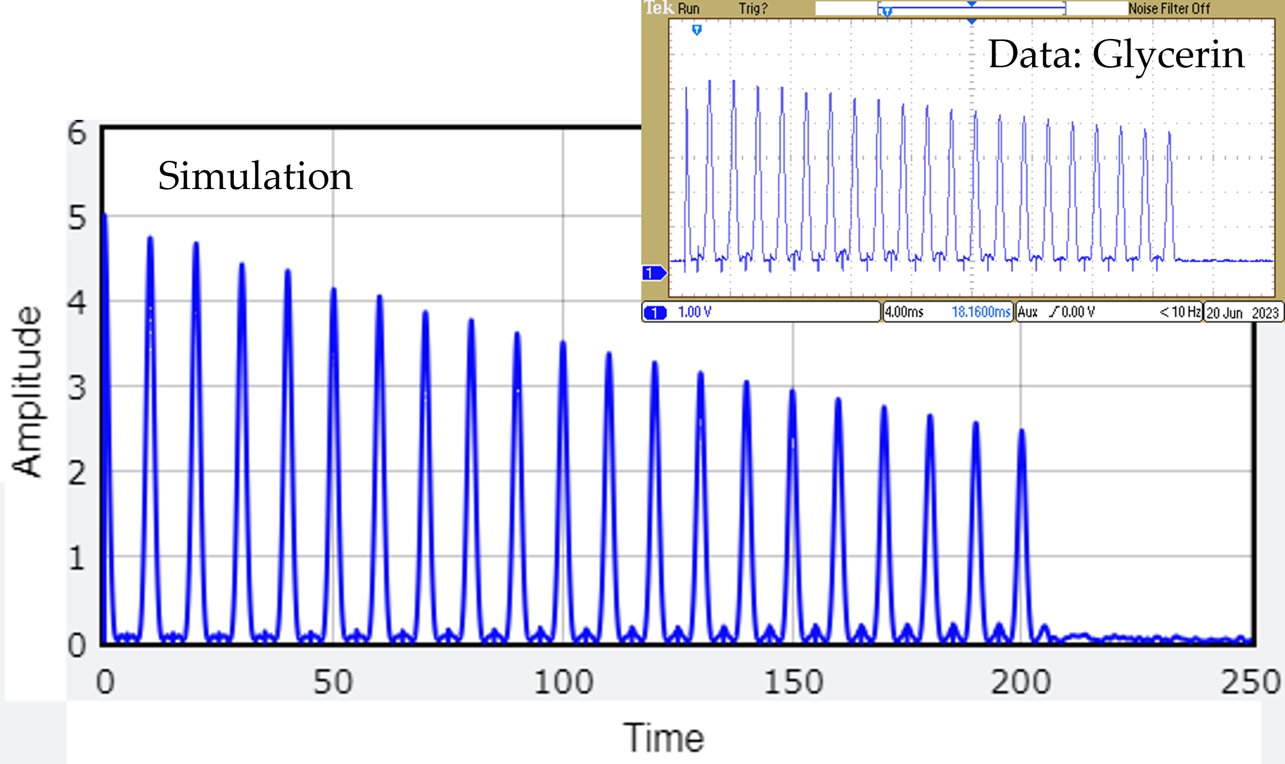
By spacing $\pi/2$ pulses so that the FID is half the height from a single pulse, one obtains the $T_1$ half-life, almost. The system recovers half of the equilibrium magnetization within a time equal to the $T_1$ half-life. This gives a correct signal for the first two pulses, but after that, the spin echo signal (1) gets tilted into the z direction (2), so $\bvec{M}_z$ evolves from that point, not the baseline, as can be seen in the simulation "data." Note the later FID pulses are higher than the initial two in both data (glycerin, above) and simulation (below).
After many pulses the ensemble forms an echo with a surprising tilted-circle configuration at the moment of the $\pi/2$ pulse. This is a steady-state configuration that reappears at every small echo peak.
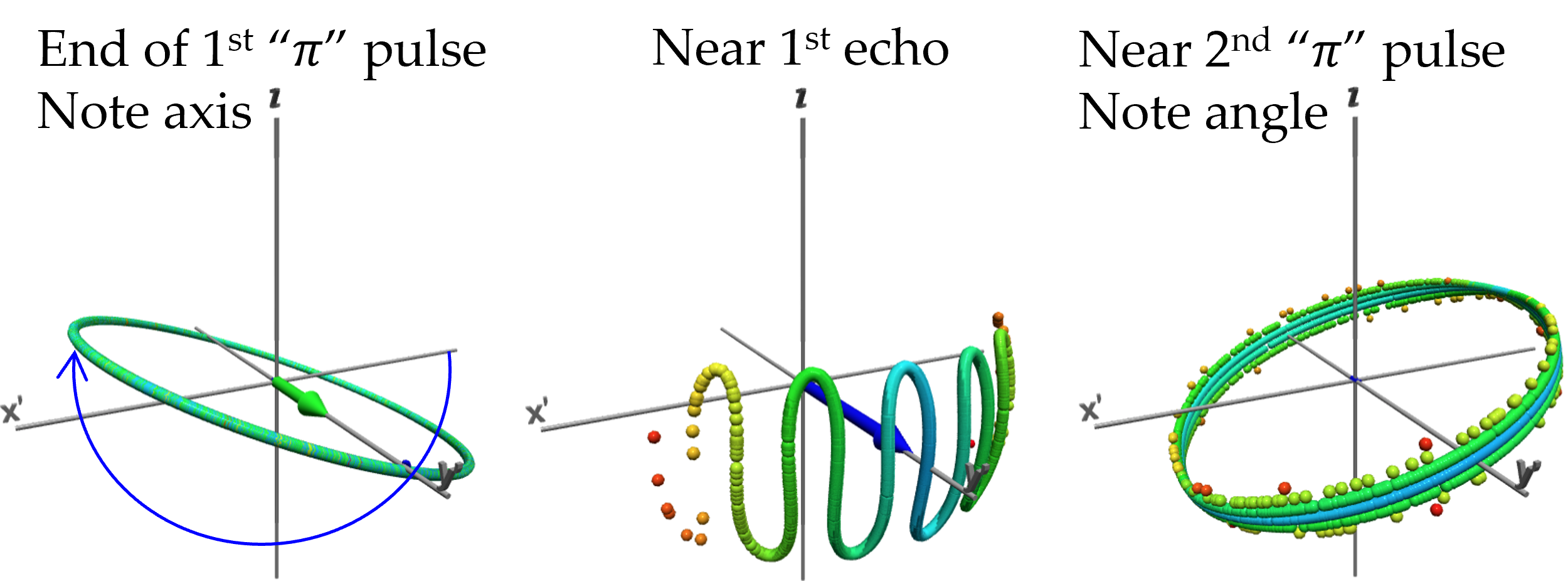
B. The canonical Carr-Purcell π/2, Nπ spin-echo sequence measurement of T2
The most common multipulse sequence, originated by Carr and Purcell, consists of a $\pi/2$ pulse followed by many ($N$) closely-spaced $\pi$ pulses. The sequence creates the easiest way to measure $T_2$ from the decay of the spin-echo envelope. The $\pi$ pulses give the strongest echoes, as the full inversion swaps the phases of the ensemble members most completely. In addition, the echo pulses are formed closest to the x', y' plane. Even if the $\pi$ pulses are more widely spaced, they still bring the ensemble back close to the x', y' plane at the time of the echo peak. The echo height is identical to the ensemble-circle’s radius.
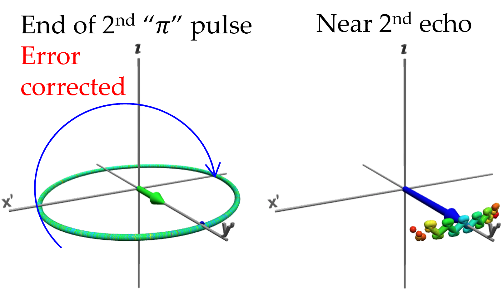
C. The Meiboom-Gill correction.
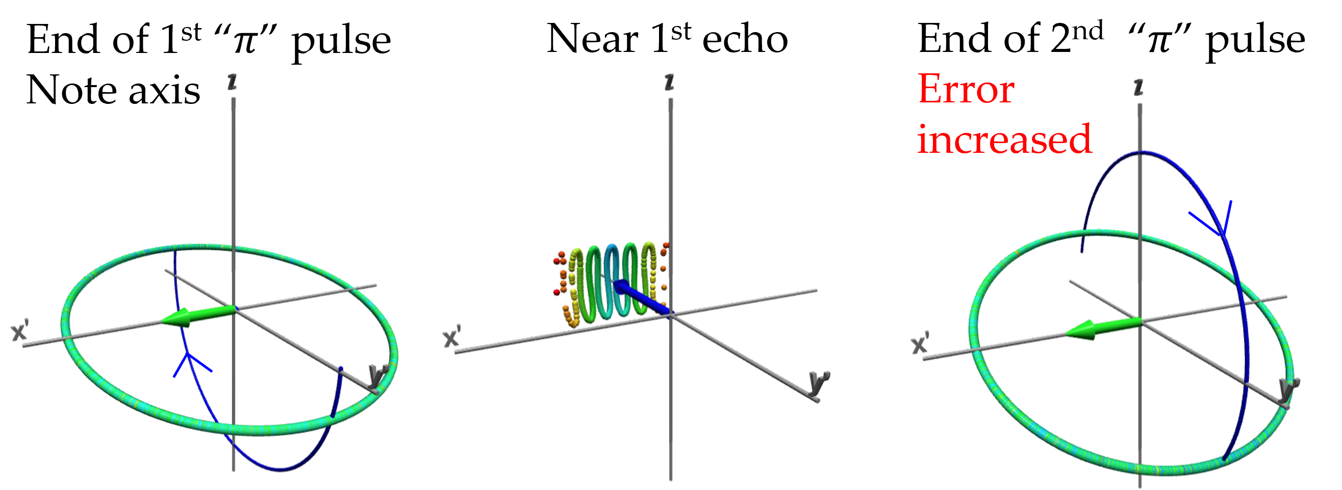
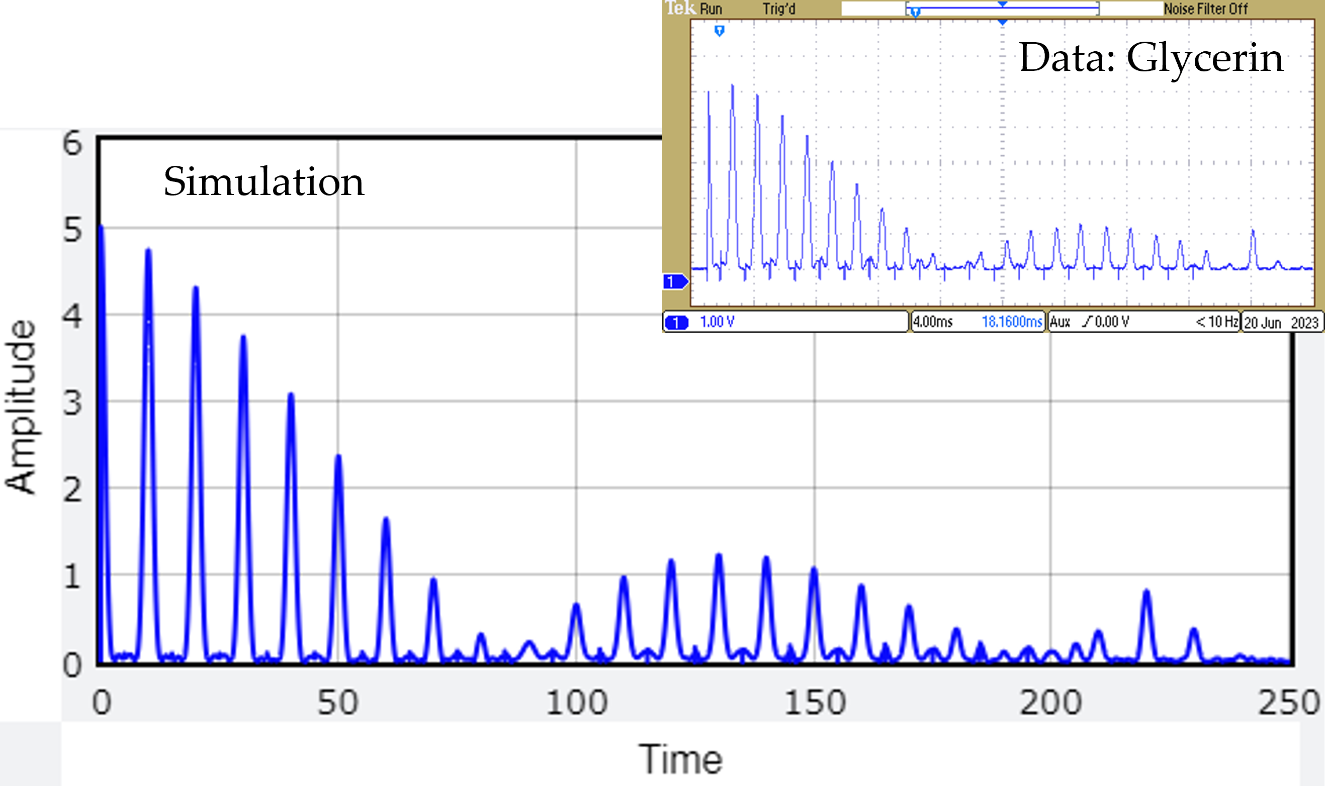
In the Carr-Purcell sequence, an error in the $\pi$-pulse width can accumulate, which makes the sequence difficult to optimize. Meiboom and Gill showed that shifting the phase of the $\pi$ pulse RF field reorients the inversion axis to be perpendicular to the axis of the original $\pi/2$ pulse, so that the accumulated error from multiple poor $\pi$ pulses is almost canceled. Even a large error can be corrected to a point. The simulation shows very clearly why the phase shift corrects the error. It also reveals the underlying geometry of the accumulated error in the absence of the M-G correction. Notice the agreement between the simulation and the data for glycerin.
M-G correction ON. In the rotating frame, $\pi$ pulses applied along the y' axis invert the ensemble about its centroid. By the time of the next pulse, the z-components have exchange positions, reversing the sign of the angle of the ensemble relative to the horizontal plane. The error is thus corrected by that pulse.
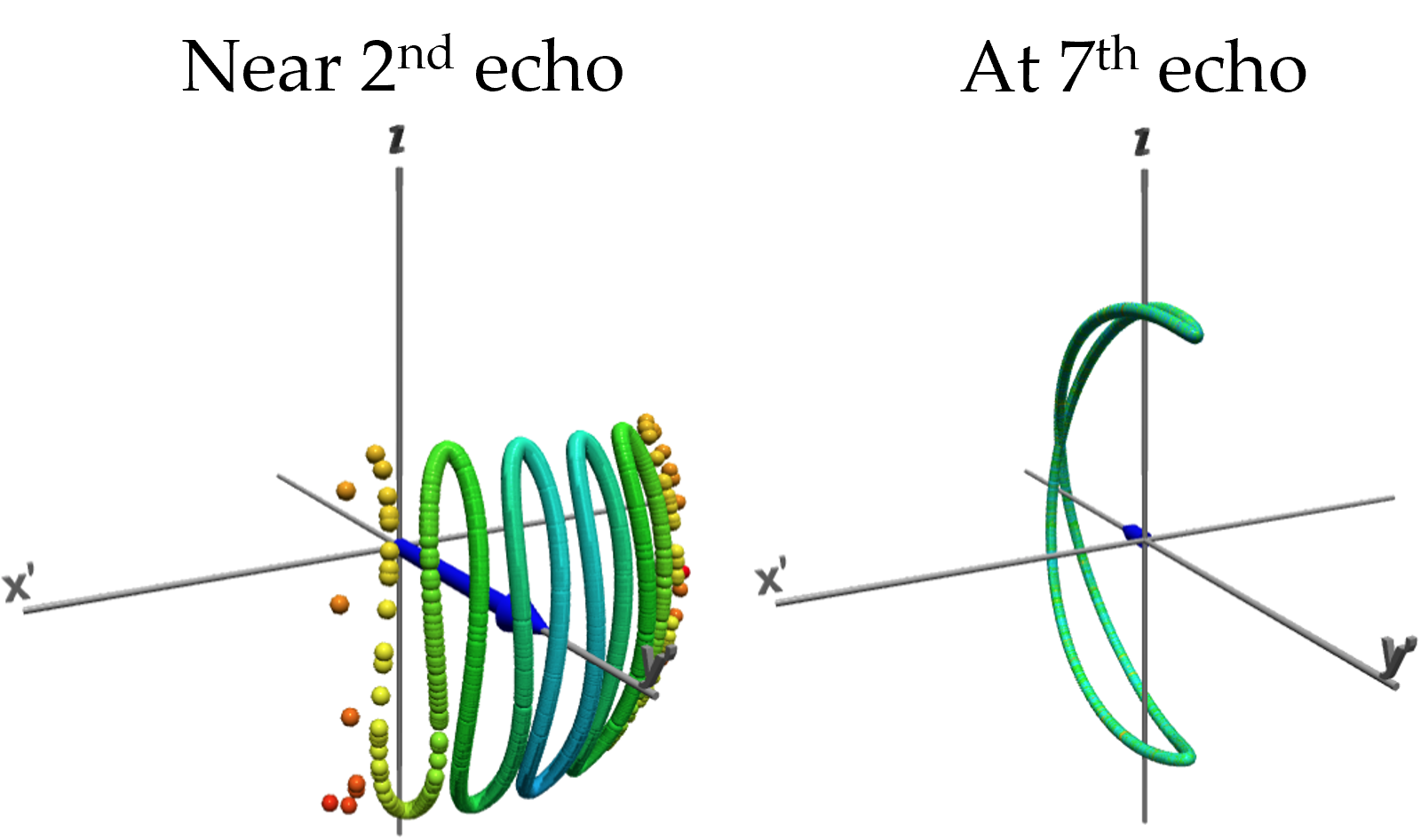
M-G correction OFF. In the rotating frame, $\pi$ pulses applied along the x′ axis invert the ensemble at its centroid, and thus the center of the ensemble, which is stationary in the rotating frame, is tilted away from the horizontal plane. Following the echo, the error in the ensemble increases with each subsequent pulse. One sees the echo envelope modulated by this error, with a larger error giving a more rapid modulation. In these images (simulated and measured) the $\pi$ pulses are about 9% too long.