2. Basics of the simulations
The computer simulations presented here were written in Python [Pérez and Granger, 2007; Ipython] using the VPython package. Developed by David Scherer, Bruce Sherwood and others, and currently maintained by Bruce Sherwood, VPython is ideally suited for rapid development of 3D physics-based animations. The browser-based Web VPython creates smooth animations by "transpiling" Python into JavaScript which is optimized for graphics in web browsers. Working versions of the programs that produced all the results shown here, plus additional information including video walk-throughs of use examples are freely available at faculty.washington.edu/dbpengra/NMR.
There is no significant challenge to simulating the Bloch equation (below), nor anything new about the computational aspects. Previous work on NMR simulation published in the American Journal of Physics has described the solution of the Bloch equation for a single-isochrome system [Grivet, 1993] and has shown how the classical descriptions of NMR arises naturally out of solving the quantum mechanical problem [Engelhardt, 2015]. My aim is to show how simulation reveals structures and patterns inherent in the Bloch equation that the NMR student may be unaware of, and to provide real-time interactive animations for students and teachers. I include comparisons to experimental data taken with apparatus in our teaching lab when possible.
Calculation of $d\bvec{M}$
\begin{equation} \label{eq:Bloch} \frac{d\bvec{M}}{dt} = -\gamma\bvec{H}\times\bvec{M} - \frac{\bvec{M}-\chi\bvec{H}}{T} \;, \end{equation}
For the simulations, which perform stepwise integration of Eq. ($\ref{eq:Bloch}$), I use the result that $-\gamma\bvec{H}\times$ operating on $\bvec{M}$ rotates $\bvec{M}$ about the direction of $\bvec{H}$ in a direction set by the right-hand rule [Jaynes, 1955]. Thus, a differential step in time $\Delta t$ for the first term of Eq. ($\ref{eq:Bloch}$) is given by $R_{\hat{H}}(-\gamma H\,\Delta t)\bvec{M}$ where $R_{\hat{H}}(\phi)$ denotes a rotation operator acting on $\bvec{M}$ about $\hat{\bvec{H}}$ through the angle $\phi=-\gamma H\,\Delta t$. The effect of the relaxation term on $\bvec{M}$ within $\Delta t$ is much smaller than from the rotation because $\gamma H \gg 2\pi/T$ (e.g., 60:1 in the simulation, or $5\times10^5:1$ in a typical apparatus, see below), so one can use a simple differential for this term. Thus, I take $\Delta\bvec{M}$ in each time step $\Delta t$ to be
\begin{equation}\label{eq:dM} \Delta\bvec{M} = R_\hat{H}(-\gamma H\,\Delta t)\bvec{M} - \left(\frac{\bvec{M}-\chi\bvec{H}}{T}\right)\Delta t\;. \end{equation}
Although it is tempting, for pedagogical purposes, to calculate the rotational differential from the cross product, in practice this can lead to an accumulating error unless $\Delta t$ is very small. Moreover, VPython's "vector" class includes a method for rotation about an arbitrary axis, making the code simple to implement.
The applied field $\bvec{H}$ is, in general, composed of two parts, a constant $\bvec{H}_0=H_0\khat$ that defines the $z$ axis, and an alternating field $\bvec{H}_1(t)$ that lies in the $x,y$ plane. Most often
\begin{equation}\label{eq:lab-frame_H1} \bvec{H}_1(t) = H_1\left(\ihat\cos\omega t - \jhat\sin\omega t\right)\;, \end{equation}
which is a circularly polarized field that rotates in the direction of precession of $\bvec{M}$ when the only field is $\bvec{H}_0$. A more common experimental form for $\bvec{H}_1(t)$ is the linearly polarized
\begin{equation}\label{eq:lab-frame_H1_linear} \bvec{H}_{1,\text{lin}}(t) = 2H_1\ihat\cos\omega t\;, \end{equation}
which has the same average magnitude as Eq. ($\ref{eq:lab-frame_H1}$). Each component of $\bvec{H}$ causes a precession of $\bvec{M}$ about its axis, and the motions combine linearly.
Parameters in simulation versus experiment
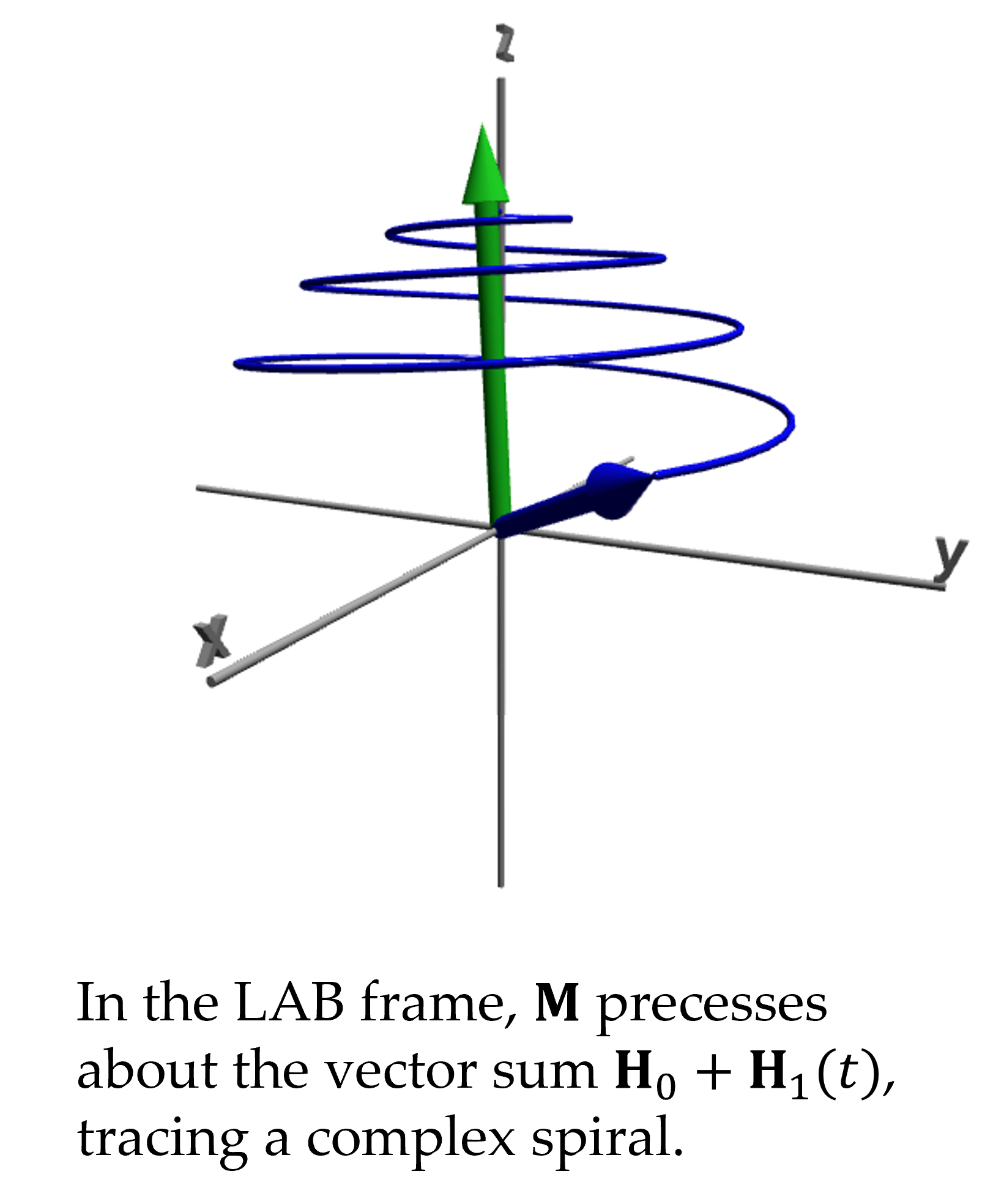
The precession angular frequency $\omega$ is directly proportional to the field magnitude, $\omega=\gamma H$. In experimental apparatus, $H_0$ is typically much larger than $H_1$. For example, in the TeachSpin PS1-A pulsed NMR unit, the precession frequency under of $\bvec{H}_0$ only, i.e., the "resonance" frequency $f_0 = \omega_0/2\pi = \gamma H_0/2\pi$ is about 15 MHz for protons, corresponding to a field of about 3500 gauss, while the amplitude of the applied RF, $H_1$, is only about 10 gauss, equivalent to $f_1=43$ kHz. In continuous-wave apparatus, which sweeps $\bvec{H}_0$ through resonance while applying the alternating field, $\bvec{H}_1$ is weaker still. The motion of the tip of $\bvec{M}$ under the combined $\bvec{H}_0+\bvec{H}_1(t)$ is thus a spherically-shaped spiral with many cycles about the $z$ axis for every cycle about an axis in the $x,y$ plane. In the PS1-A, the time it takes to invert $\bvec{M}$ from its equilibrium value of $\chi H_0\khat$ to $-\chi H_0\khat$ (about 12 μs) is the same as approximately 175 cycles around the $z$ axis. The inversion/reversion of $\bvec{M}$ is how $\bvec{H}_1(t)$ changes the energy of the system, defined as $-\bvec{M}\cdot\bvec{H}$, which is dominated by $\bvec{H}_0$.
Because the simulations aim to show the dynamics in a human readable scale, the relative sizes of the physical parameters are much closer together. $H_0$ and $\gamma$ are chosen to produce a resonant frequency of about 2 Hz, which is easily visible. The simulation shows both $\bvec{M}$ and $\bvec{H}$ vectors with $\chi=0.8$ so that both are visible with $\bvec{M}$ attaining 4/5 the length of $\bvec{H}$ at equilibrium. The oscillating field magnitude $H_1$ is much closer to $H_0$ than in a typical experiment, with values of $H_1$ in the range of $0.01H_0$ to $1.2H_0$ (the exact value of $H_1$ is user selectable). The time scale is nominally seconds, but this depends on computational speed and an adjustable rate. In the picture at left taken from one of the simulation programs, $H_1 = H_0/20$ which gives 5 cycles about the $z$ axis when $\bvec{M}$ reaches the $x,y$ plane.
The relaxation constants $T_1$, $T_2$ and $T_2^*$ are scaled to mimic typical behavior seen in liquids commonly used in student-grade NMR apparatus. For mineral oil, glycerin and water solutions of CuSO4, $T_1$ half-lives measured with the PS1-A are in the range of 10 ms for strong CuSO4 solutions up to $\approx100$ ms for glycerin. For these liquids, $T_2\approx T_1$. The $T_2^*$ parameter depends mostly on the instrument, and our PS1-A produces $T_2^*\approx1$ ms. The simulations scale these millisecond times by a factor of 1000 but keep the ratio of $T_1:T_2^{(*)}$ the same via user-selectable values from 1 to 1000 seconds for $T_1$, with $T_2$ or $T_2^*$ selected to be a percent fraction of $T_1$, depending on the application. In addition, one can turn off relaxation by setting $T_1$ and $T_2$ to "infinity". For mineral oil, which has $T_1=T_2\approx 30$ ms, the relative time constants of $T_1:T_2^*:1/f_1:1/f_0$ in the PS1-A would be approximately $3\times10^{-2}:1\times10^{-3}:2\times10^{-5}:7\times10^{-8}$ s, or $450,000:15,000:300:1$, a span of over 5 orders of magnitude. In contrast, to make all phenomena visible, the same ratio in the simulations would be $30:1:10:0.5$ s or $60:2:20:1$, only about 2 orders of magnitude. However, the ratio of the decay times to the rotational periods is misleading: first, the simulations run mostly in the rotating frame of reference, which removes $f_0$ from the picture; second, in the pulsed NMR mode, we suspend relaxation during the application of the $\bvec{H}_1$ pulse, making its time duration irrelevant.
Other aspects of the simulations are described in the following sections in the context of lessons illustrated by them.
Next: The Rotating Reference Frame