3. The rotating reference frame
Once the general character of the evolution of $\bvec{M}$ under the influence of $\bvec{H}$ is understood, the path to solution of the Bloch equation is greatly aided by transforming the coordinate system to one that rotates about the $z$ axis in the direction of $\bvec{H}_1(t)$. The simulation Bloch.py is designed to illustrate this transformation and how it indicates a need to change the form of the magnetic field to be consistent with the rotating coordinate system. The simulation allows one to select between two sets of coordinate axes, one that is fixed to the "lab" frame, and another that rotates about the $z$ axis in the same direction as the precession of $\bvec{M}$, the "rotating" frame.
Theory
To motivate the need for such a transformation, consider first a simple case of the Bloch equation in which the decay constant $T$ is large enough to allow the second term to be neglected, and that the field $\bvec{H} = H_0\khat$ only. In this approximation, the Bloch equation is
\begin{equation}\label{eq:Bloch_H0_only} \frac{d\bvec{M}}{dt} \approx -\gamma H_0\khat\times\bvec{M} = \left\{ \begin{array}{rcl} \frac{dM_x}{dt} & = & +\gamma H_0 M_y\\ \frac{dM_y}{dt} & = & -\gamma H_0 M_x\\ \frac{dM_z}{dt} & = & 0 \end{array} \right. \end{equation}
The easiest way to solve this is to define the complex quantity $M_+ = M_x + iM_y$ (and complex conjugate $M^*_+$), and from this obtain the eigenvalue equation
\begin{equation}\label{eq:M_axial_eq} \frac{dM_+}{dt} = -i\gamma H_0 M_+\;, \end{equation}
which, if we choose the initial state of $M_{+,0} = M_\perp e^{i\phi_0}= M_\perp\cos\phi_0+iM_\perp\sin\phi_0 = M_{x0}+iM_{y0} $ and set $\omega_0 = \gamma H_0$ yields the solution $M_+=M_\perp e^{-i(\omega_0t-\phi_0)}$. When transformed back to real-valued quantities, the result is
\begin{equation}\label{eq:M_H0_only_soln} \bvec{M}(t) = M_\perp\left(\ihat\cos(\omega_0 t-\phi_0) - \jhat\sin(\omega_0 t -\phi_0)\right) + M_z\khat\;. \end{equation}
Note that this result is the same as a rotation operation about the $z$ axis acting on $\bvec{M}$:
\begin{equation} \bvec{M}(t) = R_{\hat{z}}(-\omega_0 t)\bvec{M} = \begin{pmatrix} \cos\omega_0t & \sin\omega_0t & 0\\ -\sin\omega_0t & \cos\omega_0t & 0\\ 0 & 0 & 1 \end{pmatrix} \begin{pmatrix} M_\perp\cos\phi_0\\ M_\perp\sin\phi_0\\ M_z \end{pmatrix}\;, \end{equation}
which justifies the claim made in Section 2 that the result of the cross product is a rotation operation.
Now imagine changing the coordinate system to one that rides along with the rotation just described. Define two new time-varying basis vectors $\ihat^{\prime}$ and $\jhat^{\prime}$ by
\begin{align} \label{eq:prime_basis} \ihat^{\prime} & = \ihat\cos\omega t - \jhat\sin\omega t\\ \jhat^{\prime} & = \ihat\sin\omega t + \jhat\cos\omega t\nonumber\;, \end{align}
leaving $\khat$ as it is. It is clear on inspection that if $\phi_0=0$ in Eq. (\ref{eq:M_H0_only_soln}) and $\omega=\omega_0$ in Eqs. (\ref{eq:prime_basis}), then in the primed basis, $\bvec{M}(t)$ would be a constant: $M_\perp\ihat^{\prime}+ M_z\khat$. In the more general case, when $\omega\neq\omega_0$ and $\phi_0$ is nonzero, one can show that
\begin{equation}\label{eq:M_H0_only_soln_prime} \bvec{M}(t) = M_\perp\left(\ihat^{\prime}\cos[(\omega_0-\omega)t-\phi_0] - \jhat^{\prime}\sin[(\omega_0-\omega)t -\phi_0]\right) + M_z\khat\;. \end{equation}
Thus, when $\omega\rightarrow0$ the rotating frame merges with the lab frame. In the rotating frame, however, the precession speed and direction of $\bvec{M}$ depends on the difference between $\omega$ and $\omega_0$. It is useful to define a "detuning" parameter $\Delta\omega\equiv\omega-\omega_0$, and to recast Eq. (\ref{eq:M_H0_only_soln_prime}) as
\begin{equation}\label{eq:M_H0_only_Domega} \bvec{M}(t) = M_\perp\left(\ihat^{\prime}\cos(\Delta\omega t+\phi_0) + \jhat^{\prime}\sin(\Delta\omega t +\phi_0)\right) + M_z\khat\;. \end{equation}
The detuning parameter is chosen so that when the detuning is negative, $\omega\lt\omega_0$, with the retriction that $-\omega_0\le\Delta\omega$ for all reasonable values. When $-\omega_0\lt\Delta\omega\lt0$, the precession of $\bvec{M}$ in the primed frame is in the same sense as in the lab frame, but at a slower rate. At $\Delta\omega=0$ precession stops in the primed frame, and for $0\le\Delta\omega$ the precession in the primed frame is opposite that in the lab frame.
Because the precession rate and direction of $\bvec{M}$ in the rotating (primed) frame differs from that in the lab frame, the lab-frame value of $H_0$ is inconsistent with the observed motion in the rotating frame. To remedy this inconsistency, we define an "effective field" by analogy with the definition $\omega_0 =\gamma H_0$:
\begin{equation}\label{eq:effective_H0} H_{0,\text{eff}} = \frac{-\Delta\omega}{\gamma} = \frac{\omega_0 - \omega}{\gamma} = H_0 - \frac{\omega}{\gamma}\;. \end{equation}
By comparing Eqs. (\ref{eq:M_H0_only_soln}) and (\ref{eq:M_H0_only_Domega}) with the definition of $H_{0,\text{eff}}$, one can see that the Bloch equation in the rotating frame looks identical to that in the lab frame upon replacement of $H_0$ with $H_{0,\text{eff}}$. This also holds more generally; the use of the effective field in this context is similar to the concept of the coriolis force in rotational mechanics [Slichter, 1996, Ch. 2].
With the fixed field $\bvec{H}_0$, the energy does not change because it is equal to $-M_zH_0$ and $M_z$ is constant. To change the energy, there must be some field perpendicular to the $z$ axis. This is the role of $\bvec{H}_1(t)$. Within the rotating reference frame, we choose the simplest field, which would be a constant in that frame, for example $H_1\ihat^{\prime}$. In the lab frame, $\bvec{H}(t)$ would be sinusoidal in time with circular polarization:
\begin{equation}\label{eq:lab-frame_H1} \bvec{H}_1(t) = H_1\left(\ihat\cos\omega t - \jhat\sin\omega t\right)\;. \end{equation}
By specifying this form, we implicitly set the rotating frame's frequency to that of the applied $\bvec{H}_1$ field. The inclusion of $\bvec{H}_1$ modifies the effective field in an obvious way:
\begin{equation}\label{eq:H_eff} \bvec{H}_{\text{eff}} = H_1\ihat^{\prime} + \left(H_0 - \frac{\omega}{\gamma}\right)\khat\;. \end{equation}
Notice this important fact: if the frequency of $\bvec{H}_1(t)$ is equal to $\omega_0$, then the only field active in the rotating frame is $\bvec{H}_1$, and the direction of this field lies in the $x,y$ plane. This causes $M$ to precess about the $x^{\prime}$ axis, allowing for complete inversion of $\bvec{M}$ with respect to $\bvec{H}_0$ and thus the greatest energy change. This is the essence of the resonance process: when the time dependent field's frequency matches the resonant frequency of the system, it can drive strong oscillations. In this case, the oscillations are the inversion and reversion of $\bvec{M}$ along the energy-defining $\bvec{H}_0$ field.
If the frequency of the rotating field $\bvec{H}_1(t)$ does not match $\omega_0$, then by Eq. (\ref{eq:H_eff}) the effective field is tilted away from the $x,y$ plane. In the rotating frame, $\bvec{M}$ precesses about a cone defined by the angle between $\bvec{M}$ and $\bvec{H}_{\text{eff}}$. Now, a complete inversion of $\bvec{M}$ is impossible, and the energy transfer is less than on-resonance. As $\omega$ moves away from $\omega_0$, the $\khat$ component of $\bvec{H}_{\text{eff}}$ becomes dominant, and the energy transfer diminishes.
Simulating the reference frames
The simulation Bloch.py illustrates the above theory. In the simulation, the coordinate axes are "objects" that can be programmed to either stay stationary or to rotate about a vertical axis. A control allows the the choice of axes objects to display: the "lab frame" axes that are linked to $\ihat$, $\jhat$ and $\khat$, or the "rotating frame" axes that are linked to $\ihat^{\prime}$, $\jhat^{\prime}$, and $\khat$. The change in reference frame itself is literally done through a change in point of view: The visible field of the animation is defined by a "camera position" relative to the coordinate system's origin, and a "camera forward" vector that determines the direction the camera "looks." To switch between the lab frame and the rotating frame, the camera forward vector is changed from fixed to one that rotates about the $z$ axis while keeping its direction pointing toward the origin.
It is important to note that the calculation of the motion of $\bvec{M}$ and the underlying $\bvec{H}$ is unchanged when switching reference frames. However, the displayed vector representing $\bvec{H}$ is switched between $\bvec{H}$ and $\bvec{H}_\text{eff}$ by swapping $H_0\khat$ with $\left(H_0-\omega/\gamma\right)\khat$. Any change in the appearance of the $x,y$ components of $\bvec{H}$ are completely due to the change in "camera forward." The user has the option to suppress the change between $\bvec{H}$ and $\bvec{H}_\text{eff}$, and thereby see that in the rotating frame the motion of $\bvec{M}$ is inconsistent with the lab-frame vector for $\bvec{H}$.
To clearly visualize the transformation between the lab and rotating frame, execute the following steps on Bloch.py:
- the simulation and briefly turn the RF on with . This will cause the equlibrium magnetization to tilt away from the $z$ axis.
- Select Toggle axes to swap the axes from the lab (unprimed) frame to the rotating (primed) frame. You may want to slow the simulation down with Simulation speed. Notice how the rotating frame axes follow the precession of $\bvec{M}$.
- By default, the RF Detuning is set to 0, i.e., on resonance. Adjust this control and notice how the speed of the axes change, but the precession speed of $\bvec{M}$ does not.
- Switch to the rotating frame of reference with . Notice how the label changes on the button and in the lower portion of the animation frame. Now the rotating-frame axes are stopped, and the precession of $\bvec{M}$ depends on the sign and magnitude of the RF detuning $\Delta\omega$. By default, the vector display of $\bvec{H}$ switches to $\bvec{H}_\text{eff}$ when the rotating frame is active. Notice that in this case, $\bvec{H}_\text{eff}$ changes when the detuning changes, so that the precession in the rotating frame stays consistent with the effective field. Notice what happens when you toggle the axes (not the reference frame) back to the lab frame set.
-
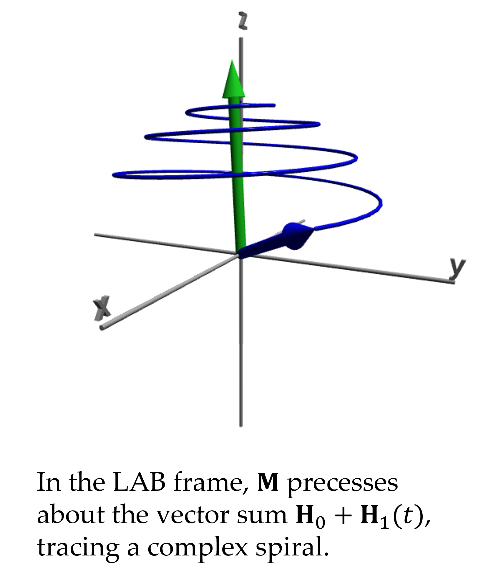
the simulation. Then , change the reference frame and axes set to show the lab frame, and select to enable $\bvec{H}_1$ again. the simulation. Notice how $\bvec{M}$ spirals toward the $-z$ axis and then back toward $+z$ over and over. Adjust RF H1 amplitude and notice how this affects the rate of inversion and reversion of $\bvec{M}$. In typical apparatus, like the TeachSpin PS1-A, the magnitude $H_1\approx0.003H_0$. See what the motion with that value looks like.
To trace the tip of $\bvec{M}$ enable its "trail" with the selection box near the top of the controls. You may also trace the tip of $\bvec{H}$ or the tip of $\bvec{M}^{\prime}$ which is the motion of $\bvec{M}$ in the rotating frame, but drawn in the lab frame. (A trail is always traced in the "home" frame of the application. In Bloch.py the home frame is the lab frame, but in Hahn.py the home frame is the rotating frame.)
As noted in Section 2 $H_1\ll H_0$.
Next: The blank