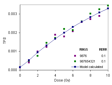
Example 16.1 Compare synthetically generated transformation frequency per survivor (TPS) data to those corresponding to the values deterministically generated by the models for different RNGS. Transformation frequency per survivor (TPS)-model generated ( rmrsim10.inp -> rmrsim10.out).Transformation frequency per survivor (TPS)-RNGS=987654321, RERR=0.1 ( rmrsim11.inp -> rmrsim11.out).  Variation of TPS with the absorbed dose for varying RNGS and constant RERR. Comments: Variation of TPS with the absorbed dose for varying RNGS and constant RERR. Comments:- Various random number generator seeds (RNGS) can be used to calculate the transformation frequency (TPS) synthetic data sets.
- The relative error is kept unchanged.
Example 16.2 Compare synthetically generated transformation frequency per survivor (TPS) data to those corresponding to the values deterministically generated by the models for different RERR. Transformation frequency per survivor (TPS)-model generated (rmrsim10.inp -> rmrsim10.out).Transformation frequency per survivor (TPS)-RNGS=9876, RERR=0.2 (rmrsim12.inp -> rmrsim12.out).  Variation of TPS with the absorbed dose for varying RERR for constant RNGS. Comments: Variation of TPS with the absorbed dose for varying RERR for constant RNGS. Comments:- Different values of the relative error (RERR) result in synthetic data with varying deviations from the model calculated values of the transformation frequency (TPS).
- RNGS is kept constant between the calculations.
Suggested problems- Compare the figures (carefully observe nature of scatter) shown in Examples 16.1 and 16.2 to understand the effects of parameters RNGS and RERR.
- Provide an example of a physical system that can be used as a random number generator (Hint: Some board games are based on simple devises that generate random numbers).
- Obtain several data points and plot a straight line of the form y = mx + c where x is the independent parameter, y is the dependent parameter, m is the slope (non zero) and c is the intercept (non zero). Then, add noise to each data point (here, you may use 5% of the y parameter and add or subtract from the y parameter value alternatively) and re-plot the x and y data. Curve fit your data with noise with a straight line and observe how well it agrees with the original straight line. This is purely a mathematical exercise (you don't need to run VC or any of its applications) designed to provide understanding of the concept of "noise". Read the introduction for more details.
- Use the input file given in example 16.1 to generate TPS data with random noise for the same relative error and different seeds (suggested: 3 different seeds). Curve fit each data set and observe how well they agree with each other, and with the same data without random noise. Discuss your results.
- Repeat problem 2 for the same seed and different relative errors (suggested: 3 different relative errors).
Tip: Experiment by changing the various model parameters and physically interpreting your results.
|


 Variation of TPS with the absorbed dose for varying RNGS and constant RERR. Comments:
 Variation of TPS with the absorbed dose for varying RERR for constant RNGS. Comments: