mmf.solve.test_problems

TwoDimensional	These are problems of two variables x and y.
Mine
MediumScale	Medium scale root-finding problems.
DennisSchnabel	Test problems from Dennis and Schnabel.

Test problems for testing non-linear solvers.

This module contains test problems with known solutions for testing non-linear solvers.

class mmf.solve.test_problems.TwoDimensional

Bases: object

These are problems of two variables x and y.

Methods

Himmelblau
MexicanHat
SensitiveParameter
test()	Test the functions.

__init__()

x.__init__(...) initializes x; see help(type(x)) for signature

class Himmelblau

Bases: object

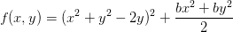
Himmelblau’s problem 2. Find the minimum of

starting from , . Solution .

Methods

F
G
J
Jinv
f
f_x
f_y

F(x, y)

G(x_)

J(x, y)

Jinv(x, y)

f(x, y)

f_x(x, y)

f_y(x, y)

class TwoDimensional.MexicanHat(a=0.5, b=0.5)

Bases: object

Classical Mexican hat potential with global minimum at , saddle point at and local maximum at where :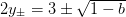

The latter two features disappear for while for the hat is completely degenerate. If is sufficiently large, then there are additional saddle points off the axis.

This becomes a very difficult problem for efficient solution when because the Jacobin becomes singular at the minimum, spoiling the quadratic convergence. This is due to the fact that function is quartic along the valley at this point as can be seen by looking at the second derivative:

Methods

F
G
J
Jinv
f
f_x
f_y

F(x, y)

G(x_)

J(x, y)

Jinv(x, y)

f(x, y)

f_x(x, y)

f_y(x, y)

class TwoDimensional.SensitiveParameter(a=1.1, b=100, c=0.1, d=0.01)

Bases: object

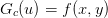
In this potential, x is a “sensitive parameter” in the sense that a good strategy is to define 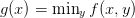and minimize this. Trying to minimize both x and y simultaneously will fail unless close to the solution.

The solution is x=y=0.

with default parameters a=1.1, b=200, c=0.1, d=0.01.

Methods

F
G
J
Jinv
f
f_x
f_y

F(x, y)

G(x_)

J(x, y)

Jinv(x, y)

f(x, y)

f_x(x, y)

f_y(x, y)

TwoDimensional.test()

Test the functions.

class mmf.solve.test_problems.Mine

Bases: object

Methods

Sqrt
test_ans()	Test the classes that the exact answer is a solution.

__init__()

x.__init__(...) initializes x; see help(type(x)) for signature

class Sqrt(*varargin, **kwargs)

Bases: mmf.solve.solver_interface.Problem

Computes the square root of two numbers with very different magnitudes. This is a simple diagonal problem, but sometimes solvers mix the two solutions causing problems. A straigh-forward application of Broyden, for example, performs very badly.

Sqrt(globals={},
     x_scale=1,
     G_scale_parameters={},
     active_parameters=set([]),
     inactive_parameters=set([]),
     n=[  1.00000000e-02   1.00000000e+02],
     start_factor=1)

Examples

>>> from mmf.solve.broyden import JinvBroyden
>>> B = JinvBroyden()
>>> p = Mine.Sqrt()
>>> x0 = p.get_initial_state().x_
>>> for n in xrange(100):
...     incompatibility = B.update(x=x0, g=p.G(x0)[0])
...     x0 = B.get_x()
>>> abs(x0 - p.ans).max() < 10
False

Attributes

class mmf.solve.test_problems.MediumScale

Bases: object

Medium scale root-finding problems.

Methods

GomexRuggiero

__init__()

x.__init__(...) initializes x; see help(type(x)) for signature

class GomexRuggiero(*varargin, **kwargs)

Bases: mmf.solve.solver_interface.Problem

These are the problems defined in Computers & Mathematics with Applications Volume 32, Issue 3, August 1996, Pages 1-13 “A numerical study on large-scale nonlinear solvers”, M. A. Gomes-Ruggiero, D. N. Kozakevich and J. M. Martinez. doi:10.1016/0898-1221(96)00109-5.

GomexRuggiero(globals={},
              x_scale=1,
              G_scale_parameters={},
              active_parameters=set([]),
              inactive_parameters=set([]),
              problem=0,
              c=0,
              n=6,
              n_0=2)

These represent a discretization of a function at equally spaced points.

The equations are the discretized form of

where is one of the following:

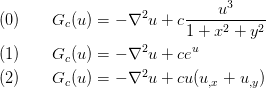
We generate the right-hand side dynamically so that the solution is exact.

Attributes

class mmf.solve.test_problems.DennisSchnabel

Bases: object

Test problems from Dennis and Schnabel.

Examples

Check that the exact answers ans are solutions:

>>> DennisSchnabel.test_ans()       
{'ExtendedPowell': True,
 'ExtendedRosenbrock': True,
 'HelicalValley': True}

Methods

ExtendedPowell
ExtendedRosenbrock
HelicalValley
Trigonometric
Wood

__init__()

x.__init__(...) initializes x; see help(type(x)) for signature

class ExtendedPowell(*varargin, **kwargs)

Bases: mmf.solve.solver_interface.Problem

The Extended Powell Singular Function.

ExtendedPowell(globals={},
               x_scale=1,
               G_scale_parameters={},
               active_parameters=set([]),
               inactive_parameters=set([]),
               m=1,
               start_factor=1)

     Note that both :math:`G` and $

abla^2 orm{G}^2` are singular at

the solution.

Attributes