mmf.math.special
| lerch_ | |
| fermi_ | |
| fermi | The core of this module is to evaluate the generalized Fermi-Dirac |
| lerch | Module of routines for computing the Lerch Trancendent and related |
| fermi_functions | Compute various properties of free fermions. |
| step(x[, x0, dx, d]) | Return the `d`th derivative of a smoothed step function. |
| LambertW(x[, k, abs_tol, rel_tol]) | Return  where where  to the desired precision. to the desired precision. |
| S(d) | Return the surface-area of a d-dimensional sphere (without the r**(d-1) factor. |
| LerchPhi(z, s, a) | Return the Lerch Trancident function  on a restricted on a restricted |
| Li(s, z) | Return the polylogarithm  . . |
| Fi(j, z) | Return the complete Fermi-Dirac integral  . . |
| fermi_integral(mu, m, T[, pmax, singlet, ...]) | Return density of a single species of free fermions of mass m |
Special Functions.
- class mmf.math.special.fermi_functions
Bases: object
Compute various properties of free fermions.
Examples
>>> fermi_functions.P(1, 1, 1)
array(0.23482812162868...)
>>> fermi_functions.N(1, 1, 1)
array(0.160318814464720...)
>>> fermi_functions.N_s(1, 1, 1)
array(0.075970412559876...)
>>> fermi_functions.dN_dmu(1, 1, 1)
array(0.193444769294...)
>>> fermi_functions.dN_dm(1, 1, 1)
array(-0.0425632327406...)
- __init__()
x.__init__(...) initializes x; see help(type(x)) for signature
- classmethod N(mu, m, T)
Return the density.
- classmethod N_s(mu, m, T)
Return the scalar density.
- classmethod P(mu, m, T)
Return the pressure.
- classmethod dN_dm(mu, m, T)
Return the derivative of the density wrt. m.
- classmethod dN_dmu(mu, m, T)
Return the derivative of the density wrt. mu.
- classmethod get_imt()
Return the class IMT instance. This is expensive to compute and so is “memoized”.
- mmf.math.special.step(x, x0=0.0, dx=0.0, d=0)
Return the `d`th derivative of a smoothed step function.
This is based on the following function
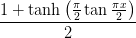
Examples
>>> import numpy as np
>>> step(-1.0)
0.0
>>> step(0.0)
0.5
>>> step(1.0, 1e-6, 1e-6/2)
1.0
>>> step(np.array(1.0), 1e-6, 1e-6/2)
1.0
The step function is implemented so that it is C(inf) smooth if dx > 0, strictly 1.0 for x > x0 + dx and strictly 0.0 for x < x0 - dx.
>>> step(np.array([0.9 - 1e-15,1.0,1.1 + 1e-15]),1.0,0.1)
array([ 0. ,  0.5,  1. ])
- mmf.math.special.LambertW(x, k=0, abs_tol=2.2204460492503131e-16, rel_tol=2.2204460492503131e-16)
Return
where to the desired precision.Parameters : x : float
k : -1, 1 or 0
Used to select the branch for x < 0.
Notes
Proceeds using the iteration:
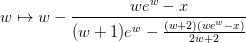
which is based on Halley’s method. Close to the solution, the absolute error is approximately:
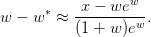
The branch
 is chosen via the initial guess. This is done with
the first two terms in the asymptotic approximation for the
non-principle branches
is chosen via the initial guess. This is done with
the first two terms in the asymptotic approximation for the
non-principle branches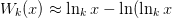
where
 and
and  is the principle
valued function. This does not work for the branches
is the principle
valued function. This does not work for the branches  and the principle branch
  near
near  and
and  . Near the
branch point we use the series approximation
. Near the
branch point we use the series approximation
where
 . If
. If  , then the positive
 is a good approximation of the
  branch, otherwise the
positive gives a good approximation for the
branch, otherwise the
positive gives a good approximation for the  branch.
For the principle branch, we use the approximation due to Winitzki??:
![W(x) \approx \frac{2\ln(1+Bp) - \ln[1 + C\ln(1+Dp)] +E}
{1+(2\ln(1+Bp) + A)^-1}](../../../_images/math/ac842334041f518a2e1234aa52d1923a8bddc9da.png)
where
 ,
,  ,
,  ,
,  , and
, and  .
.Examples
>>> LambertW(-0.2, k=0)
(-0.2591711018...
>>> LambertW(-0.2, k=1)
(-3.7223204849...+7.38723021...j)
>>> LambertW(-0.2, k=-1)
(-2.54264135777...
>>> LambertW(0.0001, k=0)
(9.9990001...
>>> LambertW(1.0,0)
(0.5671432904...
>>> LambertW(1.0,1)
(-1.533913319...+4.375185153...j)
>>> LambertW(1.0,-1)
(-1.533913319...-4.375185153...j)
>>> LambertW(1.0,2)
(-2.4015851048...+10.776299516...j)
>>> LambertW(-10.0,0)
(1.3699809685...+2.140194527...j)
Todo
Fix initial guess near 0. This does not work for k!=0 branches:
>>> W = LambertW(0.001,k=-1)
>>> np.allclose(W*np.exp(W), 0.001)
True
- mmf.math.special.S(d)
Return the surface-area of a d-dimensional sphere (without the r**(d-1) factor.
Examples
>>> S(3)
12.566370614359...
>>> S(2)
6.2831853071795...
>>> S(1)
2.0...
- mmf.math.special.LerchPhi(z, s, a)
Return the Lerch Trancident function
on a restricted
domain.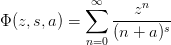
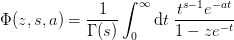
Computes the result using the integral representation
Examples
>>> abs(LerchPhi(1,2,3) - (np.pi**2/6.0 - 5.0/4.0)) < 1e-12
True
>>> abs(LerchPhi(0.5,2,3) - 0.157924211720100047221250) < 1e-12
True
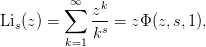
- mmf.math.special.Li(s, z)
Return the polylogarithm
.
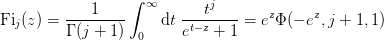
- mmf.math.special.Fi(j, z)
Return the complete Fermi-Dirac integral
.
- mmf.math.special.fermi_integral(mu, m, T, pmax=None, singlet=False, abs_tol=None, rel_tol=None)
Return density of a single species of free fermions of mass m at temperature T and chemical potential mu in natural units (
 ). Does not include any degeneracy factors:
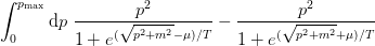
Parameters : mu : float
Chemical potential
m : float
Mass
T : float
Temperature
pmax : float
Upper limit on integration.
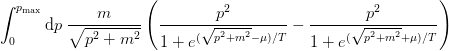
singlet : bool
If True, then the singlet density will be computed:
Examples
>>> import math, numpy as np
>>> mu = 3.0
>>> m = 2.0
>>> T = 0.0
>>> pF = math.sqrt(mu*mu-m*m)
>>> N = fermi_integral(mu, m, T)
>>> np.allclose(N, pF**3/6/pi**2)
True
>>> import math, numpy as np
>>> mu = 30.0
>>> m = 22.0
>>> T = 0.00001
>>> pF = math.sqrt(mu*mu-m*m)
>>> N = fermi_integral(mu, m, T)
>>> np.allclose(N, pF**3/6/pi**2)
True