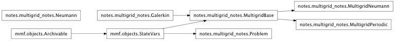
`mmf.math.multigrid.notes.multigrid_notes`¶

`Problem`(varargin, *kwargs)	Representation of the following linear problem for use with a one-dimensional multigrid method.
`Galerkin`	Provides a Galerkin operator A by interpolating and then
`MultigridBase`(varargin, *kwargs)	Common base for `MultigridNeumann` and `MultigridPeriodic`.
`MultigridPeriodic`(varargin, *kwargs)	Multigrid class for use with Periodic boundary conditions. The interpolation and restriction operators here are:
`MultigridNeumann`(varargin, *kwargs)	Multigrid class for use with Neumann boundary conditions. The interpolation and restriction operators here are:
`comparing_periodic`()	comparing the various smoothings of periodic

Inheritance diagram for mmf.math.multigrid.notes.multigrid_notes:

Inheritance diagram of mmf.math.multigrid.notes.multigrid_notes

Demo of multigrid features for multigrid.rst.

class mmf.math.multigrid.notes.multigrid_notes.Problem(*varargin, **kwargs)[source]¶

Bases: mmf.objects.StateVars

Representation of the following linear problem for use with a one-dimensional multigrid method. We provided the following problem:

Problem(a=5,
        periodic=True,
        prob=0)

$\begin{aligned} -f''(x) &= a\pi^2\left[\cos(\pi x)-a\sin^2(\pi x)\right] e^{a(\cos\pi x -1)}, \\ -f''(x) + a^2\pi^2\sin^2(\pi x)f(x) &= a\pi^2\cos(\pi x)e^{a(\cos\pi x -1)}, \\ -f''(x) - a\pi^2\cos(\pi x)f(x) &= -a^2\pi^2\sin^2(\pi x)e^{a(\cos\pi x -1)}, \\ f(x) &= e^{a(\cos\pi x - 1)}. \end{aligned}$

This can also be written as a non-linear equation:

$-f''(x) = \pi^2\left[\ln f + a - a^2\sin^2(\pi x)\right]f$

We may also write this as a set of coupled equations in a few ways, including:

$\begin{aligned} - f''(x) &= a\pi^2[g - a(1-g^2)]f, \\ - g''(x) &= \pi^2 g = \pi^2 (a^{-1}\ln f + 1) \end{aligned}$

This gives rise to the following systems for the Jacobian:

$G_3(f, g) = \begin{pmatrix} - f''(x) - a\pi^2[g - a(1-g^2)]f, \\ - g''(x) - \pi^2 g \end{pmatrix}, \qquad J_3 = -\diff[2]{}{x} + \begin{pmatrix} - a\pi^2[g - a(1-g^2)] & - a\pi^2[1 + 2g]f\\ 0 & - \pi^2 \end{pmatrix}.$

$G_4(f, g) = \begin{pmatrix} - f''(x) - a\pi^2[g - a(1-g^2)]f, \\ - g''(x) - \pi^2 (a^{-1}\ln f + 1) \end{pmatrix}, \qquad J_4 = -\diff[2]{}{x} + \begin{pmatrix} - a\pi^2[g - a(1-g^2)] & - a\pi^2[1 + 2g]f\\ - \pi^2 a^{-1}/f & 0 \end{pmatrix}.$

Attributes

class mmf.math.multigrid.notes.multigrid_notes.Galerkin[source]¶

Bases: object

Provides a Galerkin operator A by interpolating and then restricting to the top level. This is not efficient computationally, but can be used to test convergence.

Methods

A(f) Apply the operator Galerkin restriction of the operator A

__init__()¶: x.__init__(...) initializes x; see help(type(x)) for signature

A(f)[source]¶: Apply the operator Galerkin restriction of the operator A

class mmf.math.multigrid.notes.multigrid_notes.MultigridBase(*varargin, **kwargs)[source]¶

Bases: mmf.objects.StateVars, mmf.math.multigrid.notes.multigrid_notes.Galerkin

Common base for MultigridNeumann and MultigridPeriodic.

MultigridBase(n_0=2,
              n=7,
              neutralize=False,
              smoothing_method=0,
              n_smooth=[2,
              2])

Attributes

class mmf.math.multigrid.notes.multigrid_notes.MultigridPeriodic(*varargin, **kwargs)[source]¶

Bases: mmf.math.multigrid.notes.multigrid_notes.MultigridBase

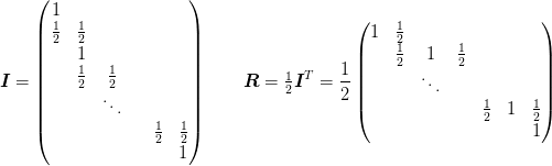
Multigrid class for use with Periodic boundary conditions. The interpolation and restriction operators here are:

MultigridPeriodic(n_0=2,
                  n=7,
                  neutralize=False,
                  smoothing_method=0,
                  n_smooth=[2,
                  2])

The restriction matrix for $n_0=2$ and $n=2\rightarrow 1$ is

$\mat{R} = \tfrac{1}{2}\mat{I}^{T} = \frac{1}{2}\begin{pmatrix} 1 & \tfrac{1}{2} & 0 & 0 & 0 & 0 & 0 & \tfrac{1}{2} \\ 0 & \tfrac{1}{2} & 1 & \tfrac{1}{2} & 0 & 0 & 0 & 0 \\ 0 & 0 & 0 & \tfrac{1}{2} & 1 & \tfrac{1}{2} & 0 & 0 \\ 0 & 0 & 0 & 0 & 0 & \tfrac{1}{2} & 1 & \tfrac{1}{2} \end{pmatrix}$

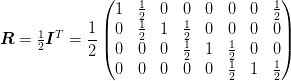
The interpolation matrix for $n_0=2$ and $n=1\rightarrow 2$ is

$\mat{I} = \begin{pmatrix} 1 & 0 & 0 & 0 \\ \tfrac{1}{2} & \tfrac{1}{2} & 0 & 0 \\ 0 & 1 & 0 & 0 \\ 0 & \tfrac{1}{2} & \tfrac{1}{2} & 0 \\ 0 & 0 & 1 & 0 \\ 0 & 0 & \tfrac{1}{2} & \tfrac{1}{2} \\ 0 & 0 & 0 & 1\\ \tfrac{1}{2} & 0 & 0 & \tfrac{1}{2} \\ \end{pmatrix}$

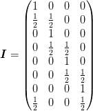
which preserve the Galerkin condition for operators of the form $T$ (yet to check)

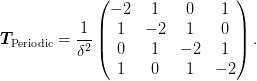
$\mat{T}_{\text{Periodic}} = \frac{1}{\delta^2}\begin{pmatrix} -2 & 1 & 0 & 1 \\ 1 & -2 & 1 & 0 \\ 0 & 1 & -2 & 1 \\ 1 & 0 & 1 & -2 \\ \end{pmatrix}.$

in the sense that $\mat{R}\mat{T}\mat{I} \simeq \mat{T}/4$ has the same tridiagonal form. In addition, the operator satisfies the symmetry and charge-neutrality conditions:

$\mat{T} = \mat{T}^{T}, \qquad \sum_{i}\mat{T}_{ij} = 0.$

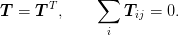
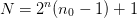
One has the following sequence of grid sizes:

$N = 2^{n}n_0$

Attributes

class mmf.math.multigrid.notes.multigrid_notes.MultigridNeumann(*varargin, **kwargs)[source]¶

Bases: mmf.math.multigrid.notes.multigrid_notes.MultigridBase

Multigrid class for use with Neumann boundary conditions. The interpolation and restriction operators here are:

MultigridNeumann(n_0=2,
                 n=7,
                 neutralize=False,
                 smoothing_method=0,
                 n_smooth=[2,
                 2],
                 inclusive=False)

$\mat{I} = \begin{pmatrix} 1\\ \tfrac{1}{2} & \tfrac{1}{2}\\ & 1 \\ & \tfrac{1}{2} & \tfrac{1}{2}\\ & & \ddots\\ & & & & \tfrac{1}{2} & \tfrac{1}{2}\\ & & & & & 1 \end{pmatrix} \qquad \mat{R} = \tfrac{1}{2}\mat{I}^{T} = \frac{1}{2}\begin{pmatrix} 1 & \tfrac{1}{2}\\ & \tfrac{1}{2} & 1 & \tfrac{1}{2}\\ && \ddots\\ & & & & \tfrac{1}{2} & 1 & \tfrac{1}{2}\\ & & & & & & 1 \end{pmatrix}$

which preserve the Galerkin condition for operators of the form

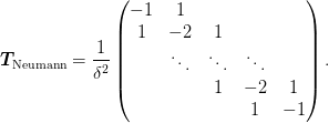
$\mat{T}_{\text{Neumann}} = \frac{1}{\delta^2}\begin{pmatrix} -1 & 1 & \\ 1 & -2 & 1\\ & \ddots & \ddots & \ddots\\ & & 1 & -2 & 1\\ & & & 1 & -1 \\ \end{pmatrix}.$

in the sense that $\mat{R}\mat{T}\mat{I} \simeq \mat{T}/4$ has the same tridiagonal form. In addition, the operator satisfies the symmetry and charge-neutrality conditions:

$\mat{T} = \mat{T}^{T}, \qquad \sum_{i}\mat{T}_{ij} = 0.$

One has the following sequence of grid sizes:

$N = 2^{n}(n_0 - 1) + 1$

Attributes

mmf.math.multigrid.notes.multigrid_notes.comparing_periodic()[source]¶: comparing the various smoothings of periodic

Previous topic

This Page

`mmf.math.multigrid.notes.multigrid_notes`¶

Navigation

Previous topic

This Page

Quick search

mmf.math.multigrid.notes.multigrid_notes¶

Navigation

`mmf.math.multigrid.notes.multigrid_notes`¶