mmf.math.multigrid.stencil
| Stencil(*varargin, **kwargs) | Represents a matrix given a stencil. |
| Interpolator(*varargin, **kwargs) | Implements an interpolation/restriction pair along a given dimension. |
| Code | Various pieces of C++ code and code generators. |
| PoissonBase | Base class for some objects representing derivatives. |
| Poisson1D | Some stencils for 1d derivatives. |
| Poisson2D | Some stencils for 2d derivatives. |
| Poisson3D | Some stencils for 3d derivatives. |
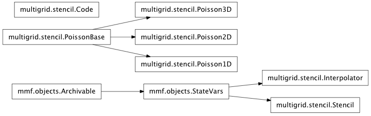
Inheritance diagram for mmf.math.multigrid.stencil:
Stencil Module (mmf.math.multigrid.stencil)
This module provides access to matrices and operators defined by a stencil.
| Stencil(*varargin, **kwargs) | Represents a matrix given a stencil. |
| Interpolator(*varargin, **kwargs) | Implements an interpolation/restriction pair along a given dimension. |
- class mmf.math.multigrid.stencil.Code[source]
Various pieces of C++ code and code generators.
- static solve(N, a_var='a', b_var='b')[source]
Return (support_code, code, libs, dirs) for solving a*x = b.
Parameters : N : int
Length of b.
a_var : str, optional
String with the name of the array a.
b_var : str, optional
String with the name of the array b.
Returns : support_code : str
Add this to the support code for weave.inline. This includes the libraries etc.
pre_code : str
Insert this near the start of your code. This allocates the array a and defines the accesser function
solve_code : str
Insert this into your code where you need to solve the system. The following must be pre-allocated and assigned:
double a[N][N];           // Done by pre_code
double b[N];
One should assign to a as a[j][[i] = a[i, j] so that Fortan order is provided as required. The result will be computed in place in the array b which m.
libs : [str]
Append these to the libraries argument for weave.inline. These are the required libs.
dirs : [str]
Append these to the linrary_dirs argument for weave.inline. These locate the libraries.
Examples
>>> a = np.array([[1, 2, 3, 4],
...               [1, 3, 5, 7],
...               [1, -2, 3, -4],
...               [1, 2, -3, -4]],  dtype=float)
>>> b = np.array([0, 1, 2, 3],  dtype=float)
>>> support_code,  pre_code,  solve_code,  libs,  dirs = Code.solve(4)
>>> code = r'''
...     %(pre_code)s
...     int i, j;
...     for (i=0;i<4;i++) {
...       for (j=0;j<4;j++) {
...         A2(i, j) = A_IN2(i, j);
...       }
...     }
...     %(solve_code)s
...     ''' % dict(pre_code=pre_code,  solve_code=solve_code)
>>> sp.weave.inline(code=code,  arg_names=['a_in',  'b'],
...                 local_dict=dict(a_in=a,  b=b),
...                 support_code=support_code,
...                 libraries=libs,  library_dirs=dirs)
>>> b
array([-3.5,   2.5,   1.5,  -1.5])
>> x = np.linalg.solve(a, b) >> y = lu_solve(a, b) >> np.allclose(a, y) True
- class mmf.math.multigrid.stencil.Stencil(*varargin, **kwargs)[source]
Bases: mmf.objects.StateVars
Represents a matrix given a stencil.
Stencil(boundary_conditions=periodic,
        S=Required)
This class uses a stencil S together with a boundary condition to represent a matrix. With extended index notation, the matrix is:

The motivation behind this was representing the Jacobian of the following system of equations:
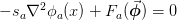
where the right-hand side is a local function of the various variables
 and the stencil
  represents the operator
 on the left-hand side. The tensor
  is
is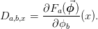
and
 is a set of scale factors.
Attributes
- class mmf.math.multigrid.stencil.Interpolator(*varargin, **kwargs)[source]
Bases: mmf.objects.StateVars
Implements an interpolation/restriction pair along a given dimension.
Interpolator(offset=0,
             boundary_conditions=periodic)
This class provides two functions I() and R() the provide interpolation and restriction functionality for a multigrid algorithm.
Examples
First we demonstrate periodic boundary conditions with the various offsets and different sized output arrays:
>>> i = Interpolator(offset=0,  boundary_conditions='periodic')
>>> f = np.array([1.0,  2.0,  3.0])
>>> i.IR(f,  (5, ))
array([ 1. ,   1.5,   2. ,   2.5,   3. ])
>>> i.IR(f,  (6, ))
array([ 1. ,   1.5,   2. ,   2.5,   3. ,   2. ])
>>> i.offset = -1
>>> i.IR(f,  (6, ))
array([ 2. ,   1. ,   1.5,   2. ,   2.5,   3. ])
>>> i.offset = 1
>>> i.IR(f,  (6, ))
array([ 1.5,   2. ,   2.5,   3. ,   2. ,   1. ])
Now we demonstrate the same with Neumann boundary conditions:
>>> i = Interpolator(offset=0,  boundary_conditions='Neumann')
>>> f = np.array([1.0,  2.0,  3.0])
>>> i.IR(f,  (5, ))
array([ 1. ,   1.5,   2. ,   2.5,   3. ])
>>> i.IR(f,  (6, ))
array([ 1. ,   1.5,   2. ,   2.5,   3. ,   3. ])
>>> i.offset = -1
>>> i.IR(f,  (6, ))
array([ 1. ,   1. ,   1.5,   2. ,   2.5,   3. ])
>>> i.offset = 1
>>> i.IR(f,  (6, ))
array([ 1.5,   2. ,   2.5,   3. ,   3. ,   3. ])
The operators are constructed explicitly so that R.T*2 == I:
>>> a = np.zeros((3, 4, 3))
>>> b = np.zeros((3, 8, 3))
>>> I = np.eye(len(b.ravel()),  len(a.ravel()))
>>> R = np.eye(len(a.ravel()),  len(b.ravel()))
>>> for n in xrange(len(a.ravel())):
...     a.flat[n] = 1
...     I[:, n] = i.IR(a,  b.shape).ravel()
...     a.flat[n] = 0
>>> for n in xrange(len(b.ravel())):
...     b.flat[n] = 1
...     R[:, n] = i.IR(b, a.shape).ravel()
...     b.flat[n] = 0
>>> abs(R.T*2 - I).max()
0.0
Attributes
State Variables: - offset
- offset : (0, -1, 1), optional
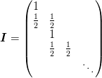
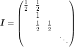
Integer offset for lower endpoint:
- offset == -1 : Here the first point depends on the
augmented array structure:
![\mat{I} = \begin{pmatrix}
\makebox[0pt][r]{\ensuremath{\tfrac{1}{2}\quad}}
\tfrac{1}{2}\\
1 \\
\tfrac{1}{2} & \tfrac{1}{2}\\
& & \ddots
\end{pmatrix}](../../../_images/math/924f26ede346c443c4e0ed46bdb3c01e9444286d.png)
- offset == 0 :
- offset == 1 :
The conditions at the right side depend on the size of the input and output arrays.
- boundary_conditions
This must be the name of one of the boundary condition transformation functions defined in support_code. Methods
IR(f, new_shape) Interpolation/restriction operator. IR_mat(shape, new_shape) Return CSR representation of the interpolation I_inline(f_in, f_out[, axis]) Interpolation operator. I_mat(shape, n_new[, axis]) Return a CSR sparse matrix representing the interpolation R_inline(f_in, f_out[, axis]) Restriction operator. R_mat(shape, n_new[, axis]) Return a CSR sparse matrix representing the restriction matrix. all_items() Return a list [(name, obj)] of (name, object) pairs containing all items available. archive(name) Return a string representation that can be executed to restore the object. archive_1([env]) Return (rep, args, imports). initialize(**kwargs) Calls __init__() passing all assigned attributes. items([archive]) Return a list [(name, obj)] of (name, object) pairs where the resume() Resume calls to __init__() from __setattr__(), suspend() Suspend calls to __init__() from This is the initialization routine. It is called after the attributes specified in _state_vars have been assigned.
The user version should perform any after-assignment initializations that need to be performed.
Note
Since all of the initial arguments are listed in kwargs, this can be used as a list of attributes that have “changed” allowing the initialization to be streamlined. The default __setattr__() method will call __init__() with the changed attribute to allow for recalculation.
This recomputing only works for attributes that are assigned, i.e. iff __setattr__() is called. If an attribute is mutated, then __getattr__() is called and there is no (efficient) way to determine if it was mutated.
Computed values with True Computed.save will be passed in through kwargs when objects are restored from an archive. These parameters in general need not be recomputed, but this opens the possibility for an inconsistent state upon construction if a user inadvertently provides these parameters. Note that the parameters still cannot be set directly.
See __init__() Semantics for details.
Methods
IR(f, new_shape) Interpolation/restriction operator. IR_mat(shape, new_shape) Return CSR representation of the interpolation I_inline(f_in, f_out[, axis]) Interpolation operator. I_mat(shape, n_new[, axis]) Return a CSR sparse matrix representing the interpolation R_inline(f_in, f_out[, axis]) Restriction operator. R_mat(shape, n_new[, axis]) Return a CSR sparse matrix representing the restriction matrix. all_items() Return a list [(name, obj)] of (name, object) pairs containing all items available. archive(name) Return a string representation that can be executed to restore the object. archive_1([env]) Return (rep, args, imports). initialize(**kwargs) Calls __init__() passing all assigned attributes. items([archive]) Return a list [(name, obj)] of (name, object) pairs where the resume() Resume calls to __init__() from __setattr__(), suspend() Suspend calls to __init__() from - __init__(*varargin, **kwargs)
This is the initialization routine. It is called after the attributes specified in _state_vars have been assigned.
The user version should perform any after-assignment initializations that need to be performed.
Note
Since all of the initial arguments are listed in kwargs, this can be used as a list of attributes that have “changed” allowing the initialization to be streamlined. The default __setattr__() method will call __init__() with the changed attribute to allow for recalculation.
This recomputing only works for attributes that are assigned, i.e. iff __setattr__() is called. If an attribute is mutated, then __getattr__() is called and there is no (efficient) way to determine if it was mutated.
Computed values with True Computed.save will be passed in through kwargs when objects are restored from an archive. These parameters in general need not be recomputed, but this opens the possibility for an inconsistent state upon construction if a user inadvertently provides these parameters. Note that the parameters still cannot be set directly.
See __init__() Semantics for details.
- IR(f, new_shape)[source]
Interpolation/restriction operator.
Interpolates (restricts) f_in along the axes where new_shape has more (fewer) elements than the corresponding dimension of f_in.
- IR_mat(shape, new_shape)[source]
Return CSR representation of the interpolation (restriction) operator along the axes where new_shape has more (fewer) elements than the corresponding dimension of shape.
- I_inline(f_in, f_out, axis=0)[source]
Interpolation operator.
Parameters : f_in, f_out : array
Pre-allocated arrays of the correct shape representing the input and output (the shape will be used to determine the upper boundary condition). These must have d dimensions. The output array need not be initialized.
axis : int, optional
Axis to perform interpolation along. (Default is 0).
Notes
This is a bit of generated C++ code that performs the action of I. The code is generated to allow for arbitrary dimensions etc. in an efficient manner. Here is an example of the completed code for a three-dimensional computation with periodic boundary conditions.
std::vector<int> i(3);
std::vector<int> j(3);
std::vector<int> j_(3);
for (i[0]=j[0]=0;i[0]<n_i[0];j[0]=++i[0]) {
  for (i[1]=j[1]=0;i[1]<n_i[1];j[1]=++i[1]) {
    for (i[2]=j[2]=0;i[2]<n_i[2];j[2]=++i[2]) {
      if (0 == (2 + i[axis] + offset)%2) {
        // Direct term
        j[axis] = (i[axis] + offset)/2;
        periodic(j,  Nf_in,  j_);
        F_OUT3(i[0], i[1], i[2]) = F_IN3(j_[0], j_[1], j_[2]);
      } else {
        // Interpolation terms
        j[axis] = (i[axis] + offset - 1)/2;
        periodic(j,  n_i,  j_);
        F_OUT3(i[0], i[1], i[2]) = 0.5*F_IN3(j_[0], j_[1], j_[2]);
        j[axis] = (i[axis] + offset + 1)/2;
        periodic(j,  n_i,  j_);
        F_OUT3(i[0], i[1], i[2]) += 0.5*F_IN3(j_[0], j_[1], j_[2]);
      }
    }
  }
}
Examples
Interpolation should always preserve constant functions:
>>> i = Interpolator(offset=0,  boundary_conditions='Neumann')
>>> f_in = np.ones((4, 3, 3, 3),  dtype=float)
>>> f_out = np.ones((4, 3, 6, 3),  dtype=float)
>>> res = i.I_inline(f_in=f_in,  f_out=f_out,  axis=2)
>>> abs(res - 1).max()
0.0
- I_mat(shape, n_new, axis=0)[source]
Return a CSR sparse matrix representing the interpolation matrix.
Parameters : shape : array
Shape of input array.
n : int
New length of interpolated axis.
axis : int, optional
Axis to perform interpolation along. (Default is 0).
Notes
This is a bit of generated C++ code that performs the action of I. The code is generated to allow for arbitrary dimensions etc. in an efficient manner. Here is an example of the completed code for a three-dimensional computation with periodic boundary conditions.
std::vector<int> i(3);
std::vector<int> j(3);
std::vector<int> j_(3);
std::vector<int> new_shape(&shape[0],  &shape[3]);
new_shape[axis] = n;
int ind = 0;
for (i[0]=j[0]=0;i[0]<new_shape[0];j[0]=++i[0]) {
  for (i[1]=j[1]=0;i[1]<new_shape[1];j[1]=++i[1]) {
    for (i[2]=j[2]=0;i[2]<new_shape[2];j[2]=++i[2]) {
      indptr[index(i,  new_shape)] = ind;
      if (0 == (2 + i[axis] + offset)%2) {
        // Direct term
        j[axis] = (i[axis] + offset)/2;
        periodic(j,  Nf_in,  j_);
        data[ind] = 1.0;
        indices[ind++] = index(j_,  shape);
      } else {
        // Interpolation terms
        j[axis] = (i[axis] + offset - 1)/2;
        periodic(j,  n_i,  j_);
        data[ind] = 0.5;
        indices[ind++] = index(j_,  shape);
        j[axis] = (i[axis] + offset + 1)/2;
        periodic(j,  n_i,  j_);
        data[ind] = 0.5;
        indices[ind++] = index(j_,  shape);
      }
    }
  }
}
indptr[index(i,  n_i)] = ind;
Examples
Interpolation should always preserve constant functions:
>>> i = Interpolator(offset=0,  boundary_conditions='Neumann')
>>> f_in = np.ones((4, 3, 3, 3),  dtype=float)
>>> f_out = np.ones((4, 3, 6, 3),  dtype=float)
>>> res = i.I_inline(f_in=f_in,  f_out=f_out,  axis=2)
>>> abs(res - 1).max()
0.0
- R_inline(f_in, f_out, axis=0)[source]
Restriction operator. Implements the transpose of I().
Parameters : f_in, f_out : array
Pre-allocated arrays of the correct shape representing the input and output (the shape will be used to determine the upper boundary condition). These must have d dimensions.
Note
The output array must be initialized to zero.
axis : int, optional
Axis to perform interpolation along. (Default is 0).
Notes
The only difference in the code from I() are:
- Exchange of f_in and f_out.
- Exchange the indices i_s with j_s.
- Turn all = into += since each output is no-longer guaranteed to be visited once. This is why we require f_out initialized to zero.
- Normalize by
 .
.
- class mmf.math.multigrid.stencil.Code[source]
Bases: object
Various pieces of C++ code and code generators.
- __init__()
x.__init__(...) initializes x; see help(type(x)) for signature
- index_support_code = '\n #include <vector>\n\n inline\n void\n periodic(const std::vector<int> &in, \n const std::vector<int> &n, \n std::vector<int> &out) {\n for (int c=0;c<in.size();++c) {\n out[c] = (in[c] + n[c]) % n[c];\n }\n };\n\n inline\n void\n Neumann(const std::vector<int> &in, \n const std::vector<int> &n, \n std::vector<int> &out) {\n for (int c=0;c<in.size();++c) {\n if (in[c] < 0) {\n out[c] = -(in[c] + 1);\n } else if (in[c] >= n[c]) {\n out[c] = 2*n[c] - in[c] - 1;\n } else {\n out[c] = in[c];\n }\n }\n };\n\n // Full parity symmetry. Only half the points in the\n // first dimension should be specified.\n //\n // (nx + 2Nx, ny + Ny, nz + Nx) = (nx, ny, nz)\n // (-nx, ny, nz) = (nx - 1, Ny - ny - 1, Nz - nz - 1)\n inline\n void\n parity(const std::vector<int> &in, \n const std::vector<int> &n, \n std::vector<int> &out) {\n int c;\n // First bring all other axes into box with periodic\n // boundary conditions.\n for (int c=1;c<in.size();++c) {\n out[c] = (in[c] + n[c]) % n[c];\n }\n\n // Now deal with x-axis\n out[0] = in[0];\n if (out[0] >= n[0]) {\n out[0] = out[0] - 2*n[0];\n }\n if (out[0] < 0) {\n out[0] = -(out[0] + 1);\n for (c=1;c<in.size();++c) {\n out[c] = n[c] - out[c] - 1;\n }\n }\n };\n\n // Symmetry consistent with sheared lattice. Includes\n // parity (Neumann boundary conditions) along the x\n // direction and parity about the origin. \n // Only half the points should be specified\n // in the first-two directions. Any shear should be\n // applied in the third dimension.\n //\n // (nx + 2Nx, ny + Ny, nz + Nx) = (nx, ny, nz)\n // (-nx, ny, nz) = (nx - 1, ny, nz)\n // (nx, -ny, -nz) = (nx, ny - 1, nz -1)\n // (nx, -ny, nz) = (nx, ny - 1, Nz - nz - 1)\n inline\n void\n shear(const std::vector<int> &in, \n const std::vector<int> &n, \n std::vector<int> &out) {\n // First bring all other axes into box with periodic\n // boundary conditions.\n int c;\n for (c=2;c<in.size();++c) {\n out[c] = (in[c] + n[c]) % n[c];\n }\n\n // Now deal with x-axis\n if (in[0] < 0) {\n out[0] = -(in[0] + 1);\n } else if (in[0] >= n[0]) {\n out[0] = 2*n[0] - in[0] - 1;\n } else {\n out[0] = in[0];\n }\n\n // Now deal with y-axis\n out[1] = in[1];\n if (out[1] >= n[1]) {\n out[1] = out[1] - 2*n[1];\n }\n if (out[1] < 0) {\n out[1] = -(out[1] + 1);\n for (c=2;c<in.size();++c) {\n out[c] = n[c] - out[c] - 1;\n }\n }\n };\n\n // Compute the linear index.\n inline\n int\n index(const std::vector<int> &i, \n const std::vector<int> &n) {\n int c;\n int res = i[0];\n for (c=1;c<i.size();++c) {\n res *= n[c];\n res += i[c];\n }\n return res;\n };\n\n // Compute the linear index with first dimension res = d.\n inline\n int\n index_d(int res, const std::vector<int> &i, \n const std::vector<int> &n) {\n int c;\n for (c=0;c<i.size();++c) {\n res *= n[c];\n res += i[c];\n }\n return res;\n };\n\n template<typename T>\n inline\n T\n prod(const std::vector<T> &x) {\n typename std::vector<T>::const_iterator iter;\n T res = 1;\n for (iter=x.begin();iter<x.end();++iter) {\n res *= *iter;\n }\n return res;\n };'
- static solve(N, a_var='a', b_var='b')[source]
Return (support_code, code, libs, dirs) for solving a*x = b.
Parameters : N : int
Length of b.
a_var : str, optional
String with the name of the array a.
b_var : str, optional
String with the name of the array b.
Returns : support_code : str
Add this to the support code for weave.inline. This includes the libraries etc.
pre_code : str
Insert this near the start of your code. This allocates the array a and defines the accesser function
solve_code : str
Insert this into your code where you need to solve the system. The following must be pre-allocated and assigned:
double a[N][N];           // Done by pre_code
double b[N];
One should assign to a as a[j][[i] = a[i, j] so that Fortan order is provided as required. The result will be computed in place in the array b which m.
libs : [str]
Append these to the libraries argument for weave.inline. These are the required libs.
dirs : [str]
Append these to the linrary_dirs argument for weave.inline. These locate the libraries.
Examples
>>> a = np.array([[1, 2, 3, 4],
...               [1, 3, 5, 7],
...               [1, -2, 3, -4],
...               [1, 2, -3, -4]],  dtype=float)
>>> b = np.array([0, 1, 2, 3],  dtype=float)
>>> support_code,  pre_code,  solve_code,  libs,  dirs = Code.solve(4)
>>> code = r'''
...     %(pre_code)s
...     int i, j;
...     for (i=0;i<4;i++) {
...       for (j=0;j<4;j++) {
...         A2(i, j) = A_IN2(i, j);
...       }
...     }
...     %(solve_code)s
...     ''' % dict(pre_code=pre_code,  solve_code=solve_code)
>>> sp.weave.inline(code=code,  arg_names=['a_in',  'b'],
...                 local_dict=dict(a_in=a,  b=b),
...                 support_code=support_code,
...                 libraries=libs,  library_dirs=dirs)
>>> b
array([-3.5,   2.5,   1.5,  -1.5])
>> x = np.linalg.solve(a, b) >> y = lu_solve(a, b) >> np.allclose(a, y) True
- class mmf.math.multigrid.stencil.PoissonBase[source]
Bases: object
Base class for some objects representing derivatives.
- __init__()
x.__init__(...) initializes x; see help(type(x)) for signature
- classmethod AB(delta_inv, boundary_conditions)[source]
Return (A, B) the stencil for the operators
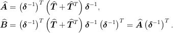
These are used as follows:
![-\pdiff{\op{\nabla}^2}{\delta_{ij}} &= \op{B}_{ij},\\
\frac{\partial^2\op{\nabla}^2}
{\partial\delta_{ij}\partial\delta_{ab}}
&= \mat{\delta}^{-1}_{ja}\op{B}_{ib}
+ \mat{\delta}^{-1}_{bi}\op{B}_{aj}
+ \left[\mat{\delta}^{-1}\left(\mat{\delta}^{-1}
\right)^T\right]_{jb}
\op{A}_{ai}.](../../../_images/math/4dbe67fbee3bad0b003c87d473005da42d180c53.png)
- d = NotImplemented
- class mmf.math.multigrid.stencil.Poisson1D[source]
Bases: mmf.math.multigrid.stencil.PoissonBase
Some stencils for 1d derivatives.
>>> Poisson1D.Laplacian
array([ 1., -2.,  1.])
- __init__()
x.__init__(...) initializes x; see help(type(x)) for signature
- Laplacian = array([ 1., -2., 1.])
- T = {(0, 0): Stencil(S=array([ 1., -2., 1.]))}
- d = 1
- class mmf.math.multigrid.stencil.Poisson2D[source]
Bases: mmf.math.multigrid.stencil.PoissonBase
Some stencils for 2d derivatives.
>>> Poisson2D.Laplacian
array([[ 0.,  1.,  0.],
       [ 1., -4.,  1.],
       [ 0.,  1.,  0.]])
# Now check that this is the same in any orthonormal basis >>> np.random.seed(0) >>> d, _R = np.linalg.qr(np.random.random((2,2))) >>> dinv = d.T >>> L = sum(dinv.T[i,j]*Poisson2D.T[j,k].S*dinv[k,i] ... for i in xrange(2) for j in xrange(2) ... for k in xrange(2)) >>> np.allclose(L, Poisson2D.Laplacian) True
- __init__()
x.__init__(...) initializes x; see help(type(x)) for signature
- Laplacian = array([[ 0., 1., 0.], [ 1., -4., 1.], [ 0., 1., 0.]])
- T = {(0, 1): Stencil(S=array([[ 0.25, 0. , -0.25], [ 0. , 0. , 0. ], [-0.25, 0. , 0.25]])), (1, 0): Stencil(S=array([[ 0.25, 0. , -0.25], [ 0. , 0. , 0. ], [-0.25, 0. , 0.25]])), (0, 0): Stencil(S=array([[ 0., 1., 0.], [ 0., -2., 0.], [ 0., 1., 0.]])), (1, 1): Stencil(S=array([[ 0., 0., 0.], [ 1., -2., 1.], [ 0., 0., 0.]]))}
- d = 2
- class mmf.math.multigrid.stencil.Poisson3D[source]
Bases: mmf.math.multigrid.stencil.PoissonBase
Some stencils for 3d derivatives.
>>> Poisson3D.Laplacian
array([[[ 0.,  0.,  0.],
        [ 0.,  1.,  0.],
        [ 0.,  0.,  0.]],

       [[ 0.,  1.,  0.],
        [ 1., -6.,  1.],
        [ 0.,  1.,  0.]],

       [[ 0.,  0.,  0.],
        [ 0.,  1.,  0.],
        [ 0.,  0.,  0.]]])
# Now check that this is the same in any orthonormal basis >>> np.random.seed(0) >>> d, _R = np.linalg.qr(np.random.random((3,3))) >>> dinv = d.T >>> L = sum(dinv.T[i,j]*Poisson3D.T[j,k].S*dinv[k,i] ... for i in xrange(3) for j in xrange(3) ... for k in xrange(3)) >>> np.allclose(L, Poisson3D.Laplacian) True
- __init__()
x.__init__(...) initializes x; see help(type(x)) for signature
- Laplacian = array([[[ 0., 0., 0.], [ 0., 1., 0.], [ 0., 0., 0.]], [[ 0., 1., 0.], [ 1., -6., 1.], [ 0., 1., 0.]], [[ 0., 0., 0.], [ 0., 1., 0.], [ 0., 0., 0.]]])
- T = {(0, 1): Stencil(S=array([[[ 0. , 0.25, 0. ], [ 0. , 0. , 0. ], [ 0. , -0.25, 0. ]], [[ 0. , 0. , 0. ], [ 0. , 0. , 0. ], [ 0. , 0. , 0. ]], [[ 0. , -0.25, 0. ], [ 0. , 0. , 0. ], [ 0. , 0.25, 0. ]]])), (1, 2): Stencil(S=array([[[ 0. , 0. , 0. ], [ 0. , 0. , -0. ], [ 0. , -0. , 0. ]], [[ 0.25, 0. , -0.25], [ 0. , 0. , 0. ], [-0.25, 0. , 0.25]], [[ 0. , -0. , 0. ], [-0. , 0. , 0. ], [ 0. , 0. , 0. ]]])), (0, 0): Stencil(S=array([[[ 0., 0., 0.], [ 0., 1., 0.], [ 0., 0., 0.]], [[ 0., 0., 0.], [ 0., -2., 0.], [ 0., 0., 0.]], [[ 0., 0., 0.], [ 0., 1., 0.], [ 0., 0., 0.]]])), (2, 1): Stencil(S=array([[[ 0. , 0. , 0. ], [ 0. , 0. , -0. ], [ 0. , -0. , 0. ]], [[ 0.25, 0. , -0.25], [ 0. , 0. , 0. ], [-0.25, 0. , 0.25]], [[ 0. , -0. , 0. ], [-0. , 0. , 0. ], [ 0. , 0. , 0. ]]])), (1, 1): Stencil(S=array([[[ 0., 0., 0.], [ 0., 0., 0.], [ 0., 0., 0.]], [[ 0., 1., 0.], [ 0., -2., 0.], [ 0., 1., 0.]], [[ 0., 0., 0.], [ 0., 0., 0.], [ 0., 0., 0.]]])), (2, 0): Stencil(S=array([[[ 0. , 0. , 0. ], [ 0.25, 0. , -0.25], [ 0. , -0. , 0. ]], [[ 0. , 0. , 0. ], [ 0. , 0. , 0. ], [ 0. , 0. , 0. ]], [[ 0. , -0. , 0. ], [-0.25, 0. , 0.25], [ 0. , 0. , 0. ]]])), (2, 2): Stencil(S=array([[[ 0., 0., 0.], [ 0., 0., 0.], [ 0., 0., 0.]], [[ 0., 0., 0.], [ 1., -2., 1.], [ 0., 0., 0.]], [[ 0., 0., 0.], [ 0., 0., 0.], [ 0., 0., 0.]]])), (1, 0): Stencil(S=array([[[ 0. , 0.25, 0. ], [ 0. , 0. , 0. ], [ 0. , -0.25, 0. ]], [[ 0. , 0. , 0. ], [ 0. , 0. , 0. ], [ 0. , 0. , 0. ]], [[ 0. , -0.25, 0. ], [ 0. , 0. , 0. ], [ 0. , 0.25, 0. ]]])), (0, 2): Stencil(S=array([[[ 0. , 0. , 0. ], [ 0.25, 0. , -0.25], [ 0. , -0. , 0. ]], [[ 0. , 0. , 0. ], [ 0. , 0. , 0. ], [ 0. , 0. , 0. ]], [[ 0. , -0. , 0. ], [-0.25, 0. , 0.25], [ 0. , 0. , 0. ]]]))}
- d = 3