`mmf.math.differentiate`¶

`differentiate`(f[, x, d, h0, l, nmax, dir, ...])	Evaluate the numerical dth derivative of f(x) using a Richardson
`D`(x[, n])	Return D where D is the nth order finite difference
`D1`(x[, sparse])	Return D where D is the finite difference
`D2`(x)	Return D2 where D2 is the finite difference
`D_Hermitian`(x[, n, boundary])	Return (D, g, ginv) where D is the nth order finite difference

Differentiation.

mmf.math.differentiate.differentiate(f, x=0.0, d=1, h0=1.0, l=1.4, nmax=10, dir=0, p0=1, err=[0])[source]¶

Evaluate the numerical dth derivative of f(x) using a Richardson extrapolation of the finite difference formula.

Parameters :

f : function

The function to compute the derivative of.

x : {float, array}

The derivative is computed at this point (or at these points if the function is vectorized.

d : int, optional

Order of derivative to compute. d=0 is the function f(x),

d=1 is the first derivative etc.

h0 : float, optional

Initial stepsize. Should be on about a factor of 10 smaller than the typical scale over which f(x) varies significantly.

l : float, optional

Richardson extrapolation factor. Stepsizes used are h0/l**n

nmax : int, optional

Maximum number of extrapolation steps to take.

dir : int, optional

If dir < 0, then the function is only evaluated to the left, if positive, then only to the right, and if zero, then centered form is used.

Returns :

df : {float, array}

Order d derivative of f at x.

Other Parameters:

p0 : int, optional

This is the first non-zero term in the taylor expansion of either the difference formula. If you know that the first term is zero (because of the coefficient), then you should set p0=2 to skip that term.

Note

This is not the power of the term, but the order. For centered difference formulae, p0=1 is the h**2 term, which would vanish if third derivative vanished at x while for the forward difference formulae this is the h term which is absent if the second derivative vanishes.

err[0] : float

This is mutated to provide an error estimate.

See also

mmf.math.integrate.Richardson(): Richardson extrapolation
Richardson(): Richardson extrapolation

Notes

This implementation uses the Richardson extrapolation to extrapolate the answer. This is based on the following Taylor series error formulae:

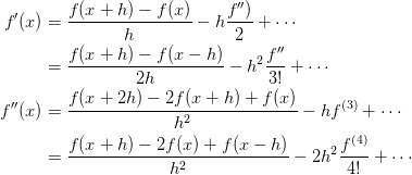
$f'(x) &= \frac{f(x+h) - f(x)}{h} - h \frac{f'')}{2} + \cdots\\ &= \frac{f(x+h) - f(x-h)}{2h} - h^2 \frac{f''}{3!} + \cdots\\ f''(x) &= \frac{f(x+2h) - 2f(x+h) + f(x)}{h^2} - hf^{(3)} + \cdots\\ &= \frac{f(x+h) -2f(x) + f(x-h)}{h^2} - 2h^2 \frac{f^{(4)}}{4!} + \cdots\\$

If we let $h = 1/N$ then these formula match the expected error model for the Richardson extrapolation

$S(h) = S(0) + ah^{p} + \order(h^{p+1})$

with $p=1$ for the one-sided formulae and $p=2$ for the centered difference formula respectively.

See mmf.math.integrate.Richardson

Examples

>>> x = 100.0
>>> assert(abs(differentiate(sin, x, d=0)-sin(x))<1e-15)
>>> assert(abs(differentiate(sin, x, d=1)-cos(x))<3e-15)
>>> assert(abs(differentiate(sin, x, d=2)+sin(x))<4e-14)
>>> assert(abs(differentiate(sin, x, d=3)+cos(x))<4e-12)
>>> assert(abs(differentiate(sin, x, d=4)-sin(x))<2e-10)
>>> differentiate(abs, 0.0, d=1, dir=1)
1.0
>>> differentiate(abs, 0.0, d=1, dir=-1)
-1.0
>>> differentiate(abs, 0.0, d=1, dir=0)
0.0

Note that the Richardson extrapolation assumes that h0 is small enough that the truncation errors are controlled by the taylor series and that the taylor series properly describes the behaviour of the error. For example, the following will not converge well, even though the derivative is well defined:

>>> def f(x):
...     return np.sign(x)*abs(x)**(1.5)
>>> df = differentiate(f, 0.0)
>>> abs(df) < 0.1
True
>>> abs(df) < 0.01
False
>>> abs(differentiate(f, 0.0, nmax=100)) < 3e-8
True

Sometimes, one may compensate by increasing nmax. (One could in principle change the Richardson parameter p, but this is optimized for analytic functions.)

The differentiate() also works over arrays if the function f is vectorized:

>>> x = np.linspace(0, 100, 10)
>>> assert(max(abs(differentiate(np.sin, x, d=1) - np.cos(x))) < 3e-15)

mmf.math.differentiate.D(x, n=2)[source]¶

Return D where D is the nth order finite difference operator over the lattice x.

Parameters :

n : int

Order. Note only n=1, 2 are reliable.

Examples

>>> x = np.cumsum(np.sin(np.linspace(0, 100, 500))**2)
>>> x = x/abs(x).max()
>>> d1 = D(x, 1)
>>> d2 = D(x, 2)
>>> f = np.sin(x)
>>> abs(np.dot(d1, f)-np.cos(x)).max() < 1e-5
True
>>> abs(np.dot(d2, f)+np.sin(x)).max() < 0.001
True

mmf.math.differentiate.D1(x, sparse=False)[source]¶

Return D where D is the finite difference operator over the lattice x.

Parameters :

type : ‘left’ | ‘center’ | ‘right’

Which type of difference formula to use for interior points.

Notes

restart;
with(CodeGeneration);
eq:={
f1=f+df*d1+ddf*d1^2/2,
f2=f+df*d2+ddf*d2^2/2};
DF:=simplify(subs(solve(eq, [df, ddf])[1], df));
simplify(coeff(DF, f));
simplify(coeff(DF, f1));
simplify(coeff(DF, f2));

eq:={
f1=f+df*d1+ddf*d1^2/2+dddf*d1^3/6,
f2=f+df*d2+ddf*d2^2/2+dddf*d2^3/6,
f3=f+df*d3+ddf*d3^2/2+dddf*d3^3/6};
DF:=simplify(subs(solve(eq, [df, ddf, dddf])[1], df));
Matlab(simplify(coeff(DF, f)));
Matlab(simplify(coeff(DF, f1)));
Matlab(simplify(coeff(DF, f2)));
Matlab(simplify(coeff(DF, f3)));

Examples

>>> x = np.linspace(0, 10, 100)
>>> d1 = D1(x)
>>> f = np.sin(x)
>>> abs(np.dot(d1, f)-np.cos(x)).max() < 0.002
True

Use sparse matrices if there is lots of data.

>>> d1s = D1(x,sparse=True)
>>> f = np.sin(x)
>>> abs(np.dot(d1, f)-np.cos(x)).max() < 0.002
True

mmf.math.differentiate.D2(x)[source]¶

Return D2 where D2 is the finite difference operator for the second derivative over the lattice x.

Notes

restart;
with(CodeGeneration);
eq:={
f1=f+df*d1+ddf*d1^2/2,
f2=f+df*d2+ddf*d2^2/2};
DF:=simplify(subs(solve(eq, [df, ddf])[1], ddf));
Matlab(simplify(coeff(DF, f)));
Matlab(simplify(coeff(DF, f1)));
Matlab(simplify(coeff(DF, f2)));

eq:={
f1=f+df*d1+ddf*d1^2/2+dddf*d1^3/6,
f2=f+df*d2+ddf*d2^2/2+dddf*d2^3/6,
f3=f+df*d3+ddf*d3^2/2+dddf*d3^3/6};
DF:=simplify(subs(solve(eq, [df, ddf, dddf])[1], ddf));
Matlab(simplify(coeff(DF, f)));
Matlab(simplify(coeff(DF, f1)));
Matlab(simplify(coeff(DF, f2)));
Matlab(simplify(coeff(DF, f3)));

eq:={
f1=f+df*d1+ddf*d1^2/2+dddf*d1^3/6+ddddf*d1^4/24,
f2=f+df*d2+ddf*d2^2/2+dddf*d2^3/6+ddddf*d2^4/24,
f3=f+df*d3+ddf*d3^2/2+dddf*d3^3/6+ddddf*d3^4/24,
f4=f+df*d4+ddf*d4^2/2+dddf*d4^3/6+ddddf*d4^4/24};
DF:=simplify(subs(solve(eq, [df, ddf, dddf, ddddf])[1], ddf));
Matlab(simplify(coeff(DF, f)));
Matlab(simplify(coeff(DF, f1)));
Matlab(simplify(coeff(DF, f2)));
Matlab(simplify(coeff(DF, f3)));
Matlab(simplify(coeff(DF, f4)));

Examples

>>> x = np.linspace(0, 10, 100)
>>> d1 = D2(x)
>>> f = np.sin(x)
>>> abs(np.dot(d1, f)+np.sin(x)).max() < 0.001
True

>>> x = np.cumsum(np.random.rand(100))
>>> x = x/x.max()*6.0
>>> d1 = D2(x)
>>> f = np.sin(x)
>>> abs(np.dot(d1, f)+np.sin(x)).max() < 0.05
True

mmf.math.differentiate.D_Hermitian(x, n=2, boundary='zero')[source]¶

Return (D, g, ginv) where D is the nth order finite difference operator over the lattice x with boundary conditions:

Parameters :

x : array of floats

Abscissa

n : int

Order of derivative

boundary : ‘zero’

Specify boundary conditions:

‘zero’: f(x[0]) = f(x[-1]) = 0

Previous topic

Next topic

This Page

`mmf.math.differentiate`¶

Navigation

Previous topic

Next topic

This Page

Quick search

mmf.math.differentiate¶

Navigation

`mmf.math.differentiate`¶