Stellar Density
Question 3: Add ln(Rho) vs. Z for stars with 0.4 < g - r < 0.6, 0.6 < g - r < 0.8, and 0.8 < g- r < 1.0 (you can rescale all curves to the same value at some ?ducial Z , or leave them as they are). Discuss the differences compared to the 0.2 < g - r < 0.4 subsample. Why do we expect larger systematic errors for 0.8 < g - r < 1.0 than for the adjacent bin with 0.4 < g - r < 0.6?
This question will show us how the number of stars varies based on their g-r color. We take the same method from question one, but now apply this to all the other g-r colors in our dataset. So we should have groups of data for 0.2 < g-r < 0.4, 0.4 < g-r < 0.6, 0.6 < g-r < 0.8, and 0.8 < g-r < 1.0. Now we have to caculate the distance for the new colors, as we had only done this for the 0.2 < g-r < 0.4 sample. Remember we need to the absolute magnitude to do this, and we need to be careful of metallicity in the larger g-r color samples, as our metallicity equation only holds for g-r < 0.6. Now we want to again create bins of 500 parsecs in terms of distance, and plot ln(Rho) vs. Z, for all colors, on the same plot. You should get a result similar to this:
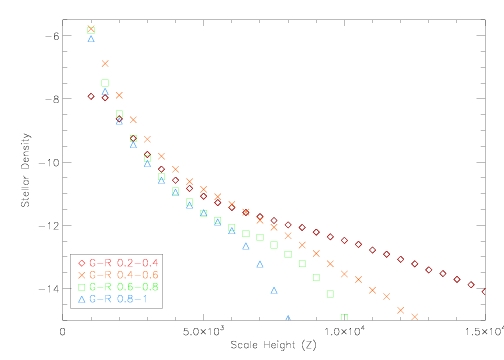
Although at very short distances several g-r colors have a higher stellar density than the 0.2-0.4 sample, they decrease at a much faster rate with respect to distance from the disk of the galaxy. The g-r samples in the0.6 < g-r < 0.8 and 0.8 < g-r < 1 color range have a larger uncertainty in their distrubution due to the fact that our metallicty equations only hold for g-r < 0.6. For these upper g-r bands we make a base assumption on their metallicity of -0.6, which may not be correct for all stars so our plots for these g-r ranges are less accurate.