Fully developed flow of polymer in a tube or between flat plates

Flow of a polymer in a tube is complicated because the viscosity is a function of shear rate, and the shear rate varies from zero at the center to a maximum at the wall. The viscosity function can be any of a number of complicated functions (link), so that the code must be robust. Here we formulate and solve the problem of the fully developed flow of a non-Newtonian fluid in a pipe or between flat plates. The orthogonal collocation method is applied to the problem, using symmetric polynomials. Since those expansions are not valid for the case of an annulus, the annulus isn't treated here. It can be treated, however, using the pipeflow examples.

Under the assumption of fully developed flow the equations are

where R is the radius of the pipe or half the distance between the two plates, and p/L is the pressure drop per unit length, which is a constant. The equation is written so that b is positive, and µ is some characteristic viscosity. The parameter a = 1 for planar geometry (flow between flat plates) and a = 2 for a pipe or cylindrical geometry. The h is the viscosity, or actual viscosity divided by µ, and it can depend on the velocity gradient. The goal is to compute the average velocity as a function of the pressure drop, or b. We integrate the equation once to obtain

where the constant of integration is set to zero to satisfy the boundary condition at r = 0. (This is where the analysis for an annulus must depart from this discussion.) We thus need to solve

when u(1) = 0 and calculate the average velocity

The viscosity function can take several forms and here we use

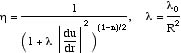
Both l₀ and n are constants characteristic of a material; different polymers have different values of the constants. The viscosity function is displayed in the figure for several choices.

For small du/dr, the viscosity is constant and we have a Newtonian fluid; the same is true if l₀ = 0 or is small. For large du/dr or large l₀ the viscosity approaches

and we have a power law fluid (link).

Next write Eq. (1) as

This is just an algebraic equation in the shear rate. For any r we can solve the equation to obtain the shear rate at that r. We then have as a function of r. Next we solve

This is a linear equation and is easily solved. The nonlinear part of the problem has been neatly compressed into a single nonlinear algebraic equation which is solved several times, once for each radial position. This solution method was suggested to the author by one of his graduate students, Thomas Patten.

The limiting behavior is useful to obtain before deriving numerical solutions. When l = 0 we have a Newtonian fluid and an analytic solution exists.

The velocity profile is a parabola. When l ­> , or du/dr ­> the problem reduces to

which has the solution

This is the solution for a power law fluid. If n is small (n ­> 0) the velocity profile is a high-order polynomial in r, and is nearly constant in the entire region except for a small boundary layer near r = 1.

The problem is solved using the orthogonal collocation method and the finite difference method.