Orthogonal collocation solution for flow of fluids in pipes, annuli, and between flat plates.
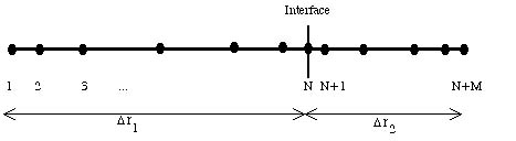
The problem is given elsewhere. The orthogonal collocation grid for this problem is shown in the figure.
There are N1 points to the left of the interface and M points to the right, giving a total of N+M points. We use the orthogonal collocation form of the equation at all points interior to the fluid, two compatibility conditions at the N-th point, and a boundary condition at the first and last point. The equations for points interior to the fluid are

The compatibility conditions are
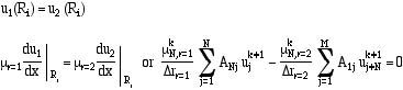
The first of these is automatically satisfied, since we use only one variable for the velocity at point N. The boundary condition at the outer boundary gives
![]()
For the inner boundary, if we have an annulus or a solid flat plate the velocity is zero.
![]()
If we have a pipe or flat plate case using symmetry the derivative is zero.
![]()
These equations represent a set of nonlinear equations (if the viscosity depends on shear rate), or a set of linear equations if the viscosity is constant in each fluid region. For the nonlinear case, we evaluate the viscosity using the shear rate at the last iteration, and then the velocity at all points is solved for simultaneously. Since the viscosity might be wrong (it was evaluated using a possibly incorrect shear rate), the viscosity is updated and the iteration continued to convergence. The form of the equations is shown in the figure.
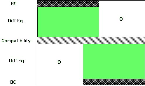
Since the orthogonal collocation method converges with N and M very rapidly, only small N and M are necessary. We could write a code to handle this shape of matrix, but it saves programming time, at the expense of increased computer time, to just use a dense matrix. The code needs the orthogonal collocation matrix programs planar.m and planar_interp.m.
The problem is solved with the interface 30% of the way between two flat plates. Region 2 (covering 70% of the space) has a viscosity that is 10 times that of region 1 (covering 30% of the space). The results with three collocation points per region are shown in the figure.
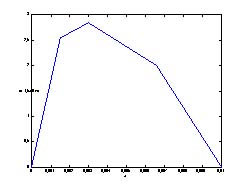
This doesn't look too promising. Results with seven collocation points per region are somewhat better.

In fact, both results are exact, and the unusual plots are due to the fact that the solution is interpolated between grid points with a straight line. If the actual polynomial is used, the results are much better.

Using a quadratic polynomial in each region (three collocation points) is sufficient to get the exact solution, which is only a quadratic function of position. Since the orthgonal collocation method is used to integrate fhe velocity, the exact flow rates are obtained for three collocation points per region, despite the straight lines in the figures. With the code shown, using the orthogonal polynomials to interpolate for the figure rather than straight lines, orthogonal collocation results are the same for any number of collocation points, from 3 to 7.
Next consider the case of a non-Newtonian fluid. Now the viscosity must be evaluated at each grid point using a subfunction. Here a made-up problem uses the formula for viscosity
![]()
Convergence of the iterations is very fast, with only xxx iterations needed. The grid refinement also shows that the numerical problem has converged to the solution of the differential equation. Note that the velocity profile is flatter over part of the region for the non-Newtonian case.
We note that we didn't need a numerical solution for two fluids with constant viscosities, but we could solve the problem numerically and compare with the exact solution. Once we had that numerical solution, though, it was relatively easy to solve for the non-Newtonian fluids, even though we could not do that analytically. Also, only minor variations were necessary to handle the pipe, annulus, or flat plates. If one used the same function for viscosity in both regions, one would get the solution for a single fluid. The only difference between this code and one for only one phase is that this code uses a compatibility condition at the N-th point, whereas a code for one phase would use the differential equation there. By running the code, you can see that this makes little difference. The orthogonal collocation method was also very much more accurate than the finite difference method, for the same number of grid points.