Polymer flow problem solved with the finite difference method

The finite difference method is also applied to Eq. (2) with a uniform grid spacing.

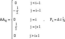
When the problem is written as

the AA matrix takes the following values for the finite difference method.

The first equation must be modified to retain the second order accuracy of the finite difference method. We can't use a false boundary (link) because there is no additional boundary condition at r = 0. Instead we use a one-side derivative (link).

Now the equations are not tridiagonal. The first two equations are

We add the second equation to the first to make the first equation:

Now the LU-decomposition routines for tridiagonal matrices can be used. In order to get the most accurate results we use Simpson's rule to calculate the average velocity. Convergence with grid refinement is shown in the table.

Flow rate for polymer flow example - finite difference method

	Trapezoid Rule			Simpson's Rule
No. Grid Points	case (a)	case (b)	case (c)	case (c)
5	0.00328168	0.757424	775.33	811.15
9	0.00332080	0.797855	1950.96	1979.64
17	0.00333057	0.807271	2446.13	2455.55
33	0.00333302	0.809534	2583.62	2589.29
65			2623.06	2623.70

A great many more points are needed in the finite difference method, compared with the method of orthogonal collocation, but the difference lessens as the velocity profile becomes flatter with more of a boundary layer.