Solution of Problem III in heat flux-temperature form with MATLAB using simultaneous solution (Version 3).

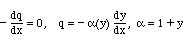
The problem to be solved is Problem III.

y(0) = 0, y(1) = 1

The finite difference formulation of this problem is

y₁ = 0, y_N = 1

When the transport coefficients at the mid-points are evaluated using the average of the points on either side, the equation becomes

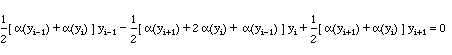
The iterative scheme is then

where the superscript k represents the value of the quantity at the k-th iteration. Thus, one takes values at the k-th iteration and calculates the values with the superscript k+1. These values are then used in the equation again, and again. The process repeats until the values no longer change, to within a specified tolerance specified by you.

These equations are applied here using MATLAB. The command file is shown below.

%solution to Problem III using version3
dx = 1;
% Solve the problem for 5 different delta-x
for kk=1:5
dx = dx/2;
n = 1 + 1/dx
% Need to iterate
tol = 1e-12;
% set up initial guess
for i=1:n
y1(i) = dx*(i-1);
end
%begin iteration
change = 1.;
iter=0;
while change>tol
iter=iter+1;
sum = 0.;
% Set up the matrices
for i=1:n
al(i) = 1+ y1(i);
end
for i=2:n-1
f(i) = 0.;
for j=1:n
aa(i,j) = 0.;
end
aa(i,i-1) = 0.5*(al(i)+al(i-1));
aa(i,i) = -0.5*(al(i+1)+2*al(i)+al(i-1));
aa(i,i+1) = 0.5*(al(i)+al(i+1));
end
% The first and last row of the matrices are special.
f(1) = 0;
f(n) = 1;
aa(1,1) = 1;
aa(1,2) = 0;
aa(n,n-1) = 0;
aa(n,n) = 1;
% Solve one iteration.
y2 = aa\f';
% Calculate the criterion to stop the iterations.
sum=0.;
for i=1:n
sum = sum + abs(y1(i) - y2(i));
y1(i) = y2(i);
end
change = sum
% Check the value of change w.r.t. tol.
end
% After convergence to within tol, save results for plotting.
nm = (n-1)/2 + 1
x=dx*(nm-1)
ys(kk) = y1(nm);
xs(kk) = dx*dx;
iters(kk)=iter
end
% Plot the value of y(0.5) versus x^2.
plot(xs,ys,'-*')
xlabel('x^2')
ylabel('y(0.5)')
clear aa
clear f
clear y1
clear y2
ys
xs
iters

The program initially sets the tolerance, grid size, and number of points. Then the first guess for y(x) is taken as a straight line. The iteration will continue until change is less than the desired tolerance. Change is defined as

Sum is the cumulative sum of absolute values of the changes in y at each node. Finally, the new value, y2, is transferred to the old value, y1, and sum is transferred to change so that the 'while' change can be tested. Finally, the last few commands print the solution and number of iterations.

How do we check our work? First, we set al(i) = 1, which is the same as taking the transport coefficient constant. In that case the solution should be a straight line, and it is. If we need to troubleshoot, we remove the ';' from the statements, use delx = 0.25, and do the calculations by hand to compare with the MATLAB results. This insures that the calculations follow the equations given above. When we have a solution, we can take the values and substitute them into the equation they are supposed to satisfy. If they do, then the equations are satisfied. You have to use judgment to decide how many of the equations you need to test; it depends on how the MATLAB program is written. Next, we solve using successively smaller ∆x and see if the solution changes. The results are all 0.58113883 (for tolerance = 10^-12). The number of iterations needed was 8, 12, 13, 13, 14, which is many fewer than the other iterative schemes, MATLAB, version 1, and MATLAB, version 2. The numbers for y(0.5) are identical so that no further analysis is necessary.

Notice that this solution is also the same derived using Excel. That is as it should be, since we are solving the same equations. The only reason for a difference is that we might not have set the tolerance to a small enough value. Needless to say, the more accurate we want the solution, the smaller is the tolerance, and the more iterations we need.

Take Home Message: Solving for all variables together makes the method converge much quicker.