Derivation of Finite Difference Method for Problem III using the Heat Flux-Temperature Formulation.
For transport problems like this one, there is another way to solve the nonlinear equations. It is convenient to use the terminology of heat transfer. The differential equation came from an energy balance involving the heat flux.
![]()
Then the heat flux was related to the temperature gradient using a constitutive equation, which in heat transfer is called Fourier's law (link).
![]()
Combination of the two equations gives equations similar to those in Problem III.
![]()
One way to solve this equation is to evaluate the transport coefficient for a chosen solution T(x). Then the boundary value problem is solved. Since the transport coefficient is possibly wrong, it is reevaluated using the newest solution, and the boundary value problem is solved again. The iteration scheme can be summarized as
![]()
For Problem III the notation is
![]()
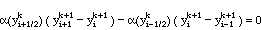
The finite difference method is applied to these equations one by one. First consider the 'energy balance', and write the finite difference expression in terms of the 'heat flux' at the mid-points to each side of the point xi, i.e. at xi + ∆x/2 and xi ∆x/2. The finite difference expression is then written using a centered derivative (link)
![]()
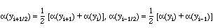
Write the constitutive equation at the mid-point, again using a centered difference expression (link).
![]()
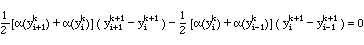
Combining these equations gives
![]()
The iterative scheme is then
How do we evaluate the transport coefficient at the mid-point, since we only have the solution at the nodes? There are several ways (link), and here we use the transport coefficient at the mid-point as the average of the transport coefficients at the two adjacent points.
The iterative scheme is then
For Problem III it is
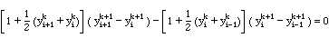
Examples of solving these equations are given when using Excel (link) and Matlab (link). The results are given in Table BVP3.
Table BVP3. Values of y(0.5) for Finite Difference Method, Problem III, Iteration Scheme No. 2
| ∆x | y(0.5) |
| 0.5 | 0.581156 |
| 0.25 | 0.5811388 |
| 0.125 | 0.5811389 |
Further calculation is not necessary. Notice that this method of solution converged to the solution (as ∆x got smaller) faster than did the first iteration scheme.