Solution of Problem III in temperature form with MATLAB using the Jacobi iteration (Version 1).
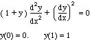
The problem to be solved is Problem III.
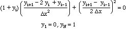
The finite difference formulation of this problem is
Rearrange the differential equation to the following form.
![]()
or
![]()
The iterative scheme can be represented as
![]()
where the superscript k represents the value of the quantity at the k-th iteration. Thus, one takes values at the k-th iteration and calculates the values with the superscript k+1. These values are then used in the equation again, and again. The process repeats until the values no longer change, to within a specified tolerance specified by you.
These equations are applied here using MATLAB. The command file is shown below.
% Solve Problem III in Matlab
tol = 1e-8;
delx = 0.0625;
n = 1/delx + 1;
y1(1) = 0;
y1(n) = 1;
% set up initial guess
for i=2:n-1
y1(i) = delx*(i-1);
end
%begin iteration
change = 1.;
iter=0;
while change>tol
iter=iter+1;
sum = 0.;
y2(1) = 0.;
y2(n) = 1.;
for i=2:n-1
y2(i) = 0.5*(y1(i+1) + y1(i-1)) + (y1(i+1)-y1(i-1))^2/(8*(1+y1(i)));
sum=sum+abs(y2(i)-y1(i));
end
% transfer y2 -> y1 for next iteration
for i=1:n
y1(i) = y2(i);
end
change = sum
% test change < tol
end
y2
iter
The program initially sets the tolerance, grid size, and number of points. Then the first guess for y(x) is taken as a straight line. The iteration will continue until change is less than the desired tolerance. Change is defined as
![]()
The expression for y2(i) is simply the iterative equation, while sum is the cumulative sum of absolute values of the changes in y at each node. Finally, the new value, y2, is transferred to the old value, y1, and sum is transferred to change so that the 'while' change can be tested. Finally, the last two commands print the solution and number of iterations.
How do we check our work? First, we remove the ';' from the statements, use delx = 0.25, and do the calculations by hand to compare with the MATLAB results. This insures that the calculations follow the equations given above. Next, we solve using successively smaller ∆x and see if the solution changes. The results are (for tolerance = 10-8):
| ∆x | y(0.5) | No. of iterations |
| 0.5 | 0.579156 | 7 |
| 0.25 | 0.58056 | 46 |
| 0.125 | 0.580986 | 190 |
| 0.0625 | 0.581100 | 738 |
A plot of y(0.5) shows that the truncation error of ∆x2 is achieved for small ∆x.
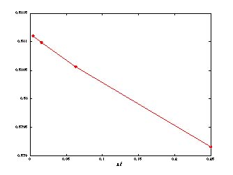
Solution to Problem III using
Finite Difference Method; plotted versus ∆x2
The numbers are close to each other. Furthermore the increments between the answers are:
(0.5, 0.25): 0.579156 0.580560 = 0.00140
(0.25, 0.125): 0.580560 0.580986 = 0.000426
(0.125, 0.0625): 0.580986 0.581100 = 0.000114
The error should go as ∆x2; with a ∆x half as big, the error should be one-fourth as big. If we are in the region (small enough ∆x) where this applies, the differences should decrease by a factor of 4 each time. In this case 0.00140 / 4 = 0.00035, which isn't quite 0.00043. However, at the next step 0.000426 / 4 = 0.000107, which is close enough to 0.000114 to say the convergence is followed. This shows that the formulas put into the spreadsheet are correct second-order expressions. Extraplolation to zero ∆x gives 0.581138.
Notice that this solution is also the same derived using Excel. That is as it should be, since we are solving the same equations. The only reason for a difference is that we might not have set the tolerance to a small enough value. Needless to say, the more accurate we want the solution, the smaller is the tolerance, and the more iterations we need.
How do we know the accuracy of our result? Firstly, we have run the problem with four different ∆x and find similar results. Secondly, we calculated the truncation error, found the error was proportional to ∆x2, and found that the results were also proportional to ∆x2 for the smallest ∆x. These two results confirm that we have solved some problem correctly. Thirdly, we carefully checked every line of the code and made sure that we solved the equation we intened to solve. Fourthly, we extrapolated the results in ∆x2 to zero to obtain the answer, 0.581138. Thus, the last calculation, with ∆x = 0.0625, was accurate to within 0.00004, or with 0.007% accuracy.
Take Home Message: Solving for a single variable in a step provides a method which is slow to converge. Version 3 is faster.