Boundary Value Problems Solved with the Finite Difference Method

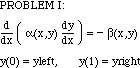
The finite difference method is illustrated by application to the following problem I, which includes heat transfer, mass transfer, and fluid flow applications.

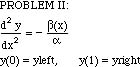
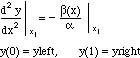
The boundary conditions are the simplest ones possible, and more complicated ones are described in other panels (link). If the function a is constant, and the function b is a function of position only, then the problem can be rewritten to form problem II.

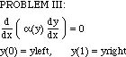
If b = 0 but a depends on the solution y in Problem I, then we get Problem III.

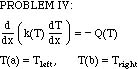
Finally, we can solve a heat transfer problem IV.

The finite difference method is applied by first dividing the domain (say x from 0 to 1) into increments as shown in the Figure BVP1.

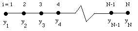
Figure BVP1. Finite Difference Mesh

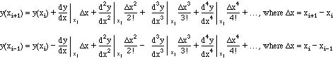
To proceed further we need to be able to write the first and second derivatives at the nodes in terms of the values at the nodes. These formulas are derived by writing a Taylor series about the point x_i.

Evaluate this at the points x_i+1 and x_i-1.

The notation can be simplified if one uses y_i = y(x_i). The equations are then

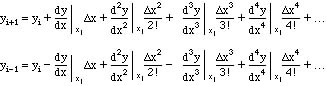
There are several ways these equations can be rearranged. First, just take y_i = y(x_i) to the left-hand side and divide by ∆x.

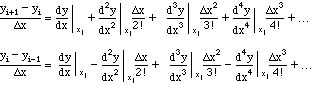
These are representations of the first derivatives at the point x_i using the values of y_i, y_i+1, or y_i­1. Now as ∆x gets small the terms multiplied by ∆x to some power will become negligible. Thus we use the following representation for the first derivatives.

These forms of the equations are sometimes called downstream and upstream derivatives, when they are used in convection problems, and the reason for the nomenclature is described when treating convection problems (link).

Remember, however, that the terms we have neglected depend on ∆x. Thus, if ∆x is not small, we have introduced an error by ignoring those terms. The error depends on the second derivative multiplied by ∆x and the third derivative multiplied by ∆x². If ∆x is small, then the error is proportional to ∆x, since the first term would be the biggest and is proportional to ∆x while the other terms are proportional to higher powers of ∆x, which are smaller numbers. Thus we call these expressions first order expressions for the first derivatives. If we knew the exact values of y at all points (i.e. no matter where x was, and no matter what ∆x was), then using a particular value of ∆x would give one estimate for the first derivative; using a ∆x half as big would give another estimate, presumably a better one. As ∆x got smaller and smaller, eventually the only term that matters would be the one multiplied by ∆x, and further decreases in ∆x would halve the error at each step if ∆x were halved each step. Unfortunately, we don't always know how small ∆x has to be for this to be the case, which makes error estimation a very important topic.

To further illustrate this effect, suppose the function y(x) is

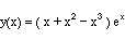
Evaluate the first derivative using the two formulas shown above. The result is shown in Figure BVP2. The upstream and downstream formula give an answer which varies linearly with ∆x, but as ∆x ­> 0, the two formulas converge on the same answer. Thus for any nonzero ∆x some error occurs, but the formula is correct in the sense that it converges to the right answer as ∆x gets smaller.

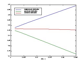
Figure BVP2. First Derivative of at x = 1.18 Using the Finite Difference Method; plots versus x

We can derive another representation for the first derivative by adding the two equations, and then rearranging them.

Thus we use the following representation for first derivative.

The error is proportional to ∆x². This representation is called the centered first derivative. An example of the error is shown in the Figure BVP2. The error is much smaller than for the case of the first order representations. From this figure it isn't apparent that the error is proportional to ∆x² for small ∆x. The data is replotted in Figure BVP3, which clearly shows this.

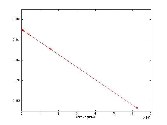
Figure BVP3. First Derivative of Using the Finite Difference Method; plots versus ∆x²

The centered first derivative has an error term that is proportional to ∆x². For small ∆x we expect the error in this representation to be proportional to ∆x²; again, though, we don't know in advance how small the ∆x has to be in order for the higher order terms to become negligible. We can determine the value by trial and error, with the assurance that it is true for small enough ∆x.

We now derive an equation for the second derivative evaluated at a grid point x_i. Add the two equations,

rearrange them, and divide by ∆x².

Thus we use for the second derivative (called a centered second derivative)

The error is proportional to ∆x², at least once ∆x gets small enough.

Continue.