Derivation of Finite Difference Method for Problem III using the Temperature Formulation.
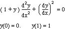
Nextapply the same methods to Problem III for the case when the transport coefficient, a, depends on the solution, y.
![]()
The equation is now more complicated, since the transport coefficient depends on the solution, too. Differentiate the equation to put it in the following form.
![]()
Here this is
Now apply the finite difference method for a certain ∆x.
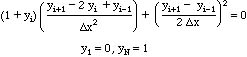
This set of algebraic equations is nonlinear, and iteration is required to solve them. However, they can be solved using analytic methods (link), Mathematica, symbolic (link), Matlab (link), or Excel (link). The results are shown in Table BVP2.
Table BVP2. Values of y(0.5) for Finite Difference Method, Problem III. Iteration Scheme No. 1
| ∆x | y(0.5) |
| 0.5 | 0.579156 |
| 0.25 | 0.58056 |
| 0.125 | 0.580986 |
| 0.0625 | 0.581100 |
A plot of y(0.5) shows that the truncation error of ∆x2 is achieved for small ∆x.
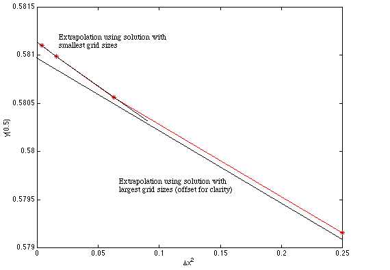
Figure BVP5. Solution to Problem III using Finite Difference Method; plotted versus ∆x2
Extrapolation (link) to zero ∆x gives 0.581138. The exact answer is (link)
![]()
and at x = 0.5 the result is 0.581139. While comparing to the exact answer is not usually an option, it is a useful exercise when learning and testing any numerical method.