From: Proceedings, SPIE - International Conference: Sensor Fusion and Decentralized Control in Robotic Systems III, Biologically Inspired Robotics, Boston, MA, Nov. 6-8, 2000, pp. 98-112.

[EDIT NOTE: This version has been edited from the original to correct some typographical and format errors. I have embedded links to my referenced papers in the text so that readers can easily find more explanations. Some references to later work are also provided so that readers can see where the research at this state led subsequently. The figures have been updated for greater clarity.]

Adapting Robot Behavior to a Nonstationary Environment: A Deeper Biologically Inspired Model of Neural Processing

George Mobus

Author's Affiliation at Time of Publication: Western Washington University
Author's Current Affiliation: University of Washington Tacoma, Institute of Technology

ABSTRACT

Biological inspiration admits to degrees. This paper describes a new neural processing algorithm inspired by a deeper understanding of the workings of real biological synapses. It is shown that a multi-time domain adaptation approach to encoding causal correlation solves the destructive interference problem encountered by more commonly used learning algorithms. It is also shown how this allows an agent to adapt to nonstationary environments in which longer-term changes in the statistical properties occur and are inherently unpredictable, yet not completely lose useful prior knowledge. Finally, it is suggested that the use of causal correlation coupled with value-based learning may provide pragmatic solutions to some other classical problems in machine learning.

Keywords: neural network, adaptive, behavior, learning, biological, robot, agent, autonomous

1. Introduction

Yet there are no principled approaches to biomimicry or theories to tell us how realistically we should try to emulate biological mechanisms[4]. The field is too new and remains exploratory. The question is: How realistic does the biomimicry need to be to achieve biological-like behavior? The field of artificial neural networks has been a study in degrees of biological inspiration. From the simple McCullough-Pitts formal neuron, inspired by gross anatomical features and the erroneous assumption that action potentials were a form of binary coding, to the more elaborate models of Grossberg and his associates[5-8], connectionist theories have variously claimed biological relevance or strong biological inspiration[9].

Then there is the issue of levels of organization. Biological entities are organized on many different levels from the chemical to the social and ecological. These levels interact in complex ways. On what level is it necessary to strive for biological realism in order to obtain biological behavior in the higher levels? There are now numerous examples of both embodied and simulated multi-agent systems in which social behaviors emerge from processes that are distinctly not biological in form or function[3, 4]. So, again, the evidence suggests that it isn’t necessary to emulate biological processes in detail to obtain the desired behaviors. However, one must also ask, how complete is the behavior repertoire being studied? Are the social behaviors observed only fragments of a complete system? If so, what sorts of problems will we have in obtaining more complete repertoires?

In this paper we examine the idea that to achieve more biologically realistic behavior at a higher level of organization requires more realism employed in emulating lower levels of organization in a biological system. We look at a single complete agent and explore the consequences of achieving higher degrees of biomimicry on three levels of organization; the synaptic and neural level, the nervous system level and the ecological survival (behavioral) level. We assert that striving for greater biomimicry on all three levels simultaneously is necessary to gain insights into the design of a complete agent. To wit, understanding the nature of the ecological/behavioral level applies important constraints on the options explored in the nervous system and neural levels. At the same time, neural processing determines what can be explored at the nervous system and behavioral levels. Here we will present one of the levels, the neural level, in some detail and the other two to a lesser extent, owing to the constraints of the venue.

Specifically, we present an adaptive mechanism, which more closely follows both the form and function of real biological synapses, and discuss some of the advantages of using this mechanism in developing a neural controller for an embodied autonomous agent. We show how a new dynamic synapse model solves a long-standing problem in encoding causal relations in a nonstationary environment, namely the destructive interference problem. We further show how this mechanism is employed in a neurally based control architecture for a robot. That architecture implements a form of value-based learning[4] (pp 469-474 & 493-498).

Finally, we discuss some general features of the architecture we have developed using this neural system and how it is used in an embodied agent — the MAVRIC robot. We describe the task environment (ecology) we are developing to test its capacity to produce animal-like adaptive behavior in an open, nonstationary world. Following the same philosophy of more closely emulating biological processes, we are constructing a foraging task environment that is open and in which relationships between objects are subject to nonstationary stochastic change.

2. Dynamic Synapses

Recently considerable interest has been shown in a class of synaptic encoders called dynamic synapses, used in unsupervised or self-supervised learning. These encoders differ from classical ANN learning rules, which describe a procedure whereby a synaptic efficacy weight evolves toward some fixed-point in the course of learning. These latter types of rules have found successful application in problems in pattern learning, identification and classification and optimal control[10, 11]. But they operate on the assumption that an environment is essentially stationary. That is, the underlying assumption is that the statistical properties of the environment — the relations between elements in the pattern(s) — remain fixed. It is the job of the neural network to extract these relationships from experience. Once a pattern (or category) is learned, it is assumed that it will remain a valid pattern for the life of the network.

Dynamic synapses are predicated on the notion that forgetting is as important as learning. That is, the underlying assumption is that the environment is not stationary (c.f. [12, 13]), though it must be sufficiently stable over the life of the agent so that what is learned is useful. In these synapses the efficacy response of the synapse may vary in time, both up and down, depending on the history of excitation and, possibly the history of correlated feedback. One of the first investigations of this type of synaptic mechanism was by Alkon, et al.[2] in the Dynamo model. This model was based on Alkon’s earlier investigations of real biological synapses and memory trace phenomena in both invertebrate and mammalian nervous systems[14], discussed further below. Those investigations introduced the notion of time domains in evolving synaptic efficacy. That is, the response characteristic of a synapse — the post-synaptic excitatory potential (EPSP) — is modulated in multiple time scales by various coupled biochemical processes in the post-synaptic compartment.

There is an unfortunate consequence of using single time scale forgetting to allow continuous learning in a nonstationary world. Passive forgetting, just due to the passage of time without signal reinforcement, falls off exponentially as fast as the memory trace encoded in synaptic efficacy increased (see below). In the case of active forgetting, e.g., due to learning new correlations, an old association is sacrificed to accommodate the new one, a problem designated as “destructive interference”. In both cases old memory traces are eliminated regardless of how useful the encoded memory trace had been over the period it was formed. This means that if the new condition is actually transient with respect to the lifetime of the agent, useful knowledge is lost. It is true that the agent can always relearn the older association, again at the expense of the newer one. But this is both inefficient and potentially detrimental to the behavior of the agent.

Animals do not completely forget prior learned associations. Suppose an animal is conditioned that a specific cue event is followed by a reward — food. After so many pairings of the cue and reward the animal reacts to the cue as if the reward were already presented. If this protocol is continued over an extended time scale the animal forms a deep association that can be retrieved even after a long period of non-occurrence. Subsequently, if the animal is subjected to several episodes of the cue being paired, not with reward, but with pain instead, the animal will quickly learn the new association and react to the cue as if it always preceded a painful encounter. From this behavior it might be concluded that the animal actively forgot the cue-reward association and the cue-pain association has destroyed the older one. But in fact it can be shown that with the passage of time where episodes of the cue are not followed by pain (and not even necessarily by reward), the animal’s aversive reaction to the cue will fade and, in a few cases, the reward expectation behavior will re-emerge in a weak form. More generally, if the animal is subsequently exposed to cue-reward pairing episodes, the older association will be “relearned” much more rapidly than it took to learn it the first time. In other words the memory trace of the older association had not been destroyed. A more recent, and hence more salient, association had only masked it. The phenomenon is known as “savings” in the animal learning literature. The multi-time domain model of efficacy modulation can explain this phenomenon[14-18].

3.Biological Synapses

Synaptic efficacy in most ANN models has been based on a single weight computed as the correlation between input and output activity (Hebbian rule)[19] or input and error (delta-rule, backpropagation)[10, 11]. These models are simple and effective in standard pattern learning or classification problems. They are not necessarily biologically realistic. Moreover they suffer from inherent problems with respect to long-term memory versus short-term learning. Fast learning gives rise to fast forgetting. Conversely slow learning does not allow an agent to adapt rapidly enough to many real world situations. Real synapses display multiple time scale modulation, are capable of fast short-term learning and very long-term memory retention.

From the neurobiological evidence it is clear that real synaptic efficacy has a complex dynamic dependent on many factors [14, 15, 20-26]. Activity-dependent and secondary factor modulation gives rise to response characteristics quite different from simplistic models. Specifically, the response of a biological synapse is the degree of depolarization (or hyperpolarization) that that synapse contributes to the local dendritic or cell body membrane. Synapses, even ones that are involved in well-established short-term memory traces, are known to produce initial weak responses to single action potential spikes in very low frequency spike trains. This may allow the synapse to filter out low-level noise or spontaneous spiking. If spiking rates, even moderately low, are sustained however, the excitatory (or inhibitory) post-synaptic potential or EPSP (a trace of the synapse’s response) rises further on each subsequent spike. The synapse undergoes an activity-dependent increase in its efficacy.

Potentiation is the phenomena whereby an EPSP becomes not only elevated but does not decay back to the full resting potential after the input signal is reduced. Studies show that tetanic stimulation (high frequency episodic spiking) results in a sustained elevation of resting potential[22]. Additionally, studies of associative long-term potentiation show that such elevation may last for very long periods (days, weeks) when paired properly with a secondary signal. Alkon has elucidated a number of biochemical pathways within the post-synaptic compartment, which have temporal properties of the right character to explain the multi-time domain potentiation seen in these synapses[14]. It is beyond the scope of this paper to delve into this model in any detail here. Interested readers are encouraged to read the references. Of relevance here is that dynamic synapses are often modeled using simple leaky integrator dynamics[25]. Real synapses, however, have behavior that departs significantly from a simple exponential decay (ibid).

The behavior of a biological synapse can be explained by the introduction of a multi-time domain model. Figure 1 shows a summary of such a model, taken largely from Alkon[14]. The figure shows a pre-synaptic bouton and a post-synaptic compartment for two neighboring synapses. Alkon related the synaptic mechanisms for encoding a memory trace to the behavioral aspects of a whole animal (a marine nudibranch) that he showed was subject to classical conditioning. Demonstrating the correspondence between memory trace mechanisms and whole animal behavior has significant consequences for the development of embodied artificial agents. In the figure one synapse is associated with the conditioned stimulus input (CS) and the other with the unconditioned stimulus (UCS). Not shown directly is the fact that the EPSP or response of the UCS synapse gives rise to the unconditioned response or output from the neuron. On conditioning, the depolarization response of the CS synapse similarly generates the unconditioned response since both synapses are within the same neuron. The figure shows a series of increasing time domains (from instantaneous response to days and possibly years — in the case of higher organisms).

Briefly, an arriving spike at the CS input causes a transient rise in the EPSP of the post-synaptic membrane; the essentially instantaneous depolarization. This depolarization leads to an influx of calcium ions, but quick recovery of the polarization of the membrane will limit the influx and its subsequent consequences. In this model a time-delayed input in the UCS synapse leads to higher local depolarization of the local membrane region. This allows a greater influx of calcium ions into the post-CS compartment. The consequence of a higher calcium concentration is a decrease in potassium ion outflux which, in turn, leads to a higher EPSP response on subsequent inputs to the CS synapse. Thus, the input of a UCS signal shortly after the onset of the CS signal leads to a short time-scale potentiation of the CS synapse. It is important to note that if the time order of signals is reversed, that is UCS onset comes before CS onset, the CS synapse will actually be depressed leading to a blockage of calcium influx and no potentiation. In this way, the synapse is prevented from “recording” a non-UCS signal as a CS when, in fact, it does not precede the UCS. A true CS-UCS relation is important because a CS (bell ringing in the Pavlov experiments) acts as a predictor of the biologically important event, the UCS (food presentation).

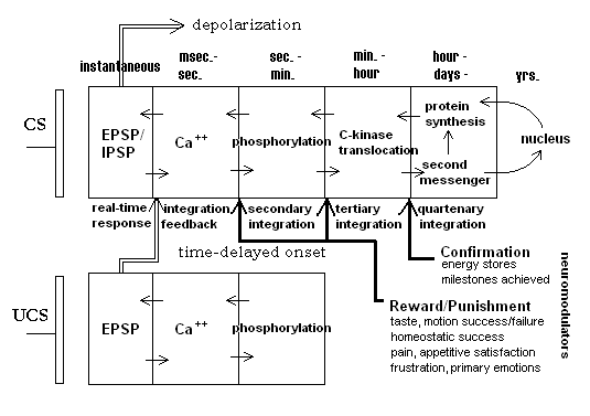
Figure 1. Temporally-ordered, quasi-hebbian synapse. Diagram shows increasing time domains. Domains are gated by neuromodulator feedback from longer time-frame processes. After Alkon, 1987.

Alkon’s model goes on to outline latter stages in the post-synaptic processes that lead to further and longer-sustained potentiation. In the figure, calcium concentration also initiates the longer-term phosphorylation (removal of a phosphate group from a protein molecule leading to inactivation of that molecule) of potassium ion channels. Longer still, the translocation of C-kinase, an enzyme, from the cytosol into the post-synaptic membrane sustains this phosphorylation. The long-term potentiation is thought to further initiate second messenger processes which influence both protein synthesis rates and possibly the rate and kind of mRNA production from the nucleus. These later processes could have really long-term consequences for the efficacy of the synapse. In the last case, for example, it could result in increases in the number of neurotransmitter receptor sites in the post-synaptic membrane.

The UCS synapse is not, technically, a learning or adaptive synapse. It does show nonlinear dynamic activity-dependent response behavior, but does not necessarily show the long-term potentiation shown by the CS synapses. Its role is to unconditionally generate an action potential (or more) in the neuron and to gate potentiation in any nearby adaptive synapses that had very recently been excited. Alkon, et al. calls this type a “flow-through” synapse[2].

Finally, note that the deeper stages in the CS synapse may themselves be gated by longer-term feedback from a number of sources within the animal. Events under the rubric “Reward/Punishment” produce evaluative feedback to the synapse through neuromodulators (broadcast signals). This happens within a short time after behavior. It is assumed that rewarding signals such as might be generated from experiencing a good taste after putting some presumptive food into the mouth will gate potentiation to the next stage. Punishing results should prevent potentiation and possibly even shunt previous stages, e.g., lead to increased calcium-sequestering processes. “Confirmation” feedback arrives much later, coming from such conditions as satiation, or longer still, from physiological signals, say from the liver or fat cells, indicating higher levels of reserve energy stores. Speculatively, such an organization of gating over multiple time domains could provide an answer to the credit-assignment problem. Those traces that contributed to actions leading to an eventual global reward would be elevated by virtue of potentiation of the intermediate levels, themselves each rewarded in their own time scale.

The exact biochemical details of these mechanisms are still only poorly understood. But the broad outline of the time-course behavior of this system is fairly well established. It should be noted that this model also accounts for the Hebb rule indirectly. In the plain-vanilla version of the Hebb rule, the change in synaptic weight is a function of the correlation of the input with the neuron output. In the Alkon model it is the time-oriented association of two input signals, one of which is guaranteed to generate an output from the neuron, rather than the simple correlation between an input (resulting from the output of an upstream neuron) and the output of a neuron that results in strengthening the input synapse. A casual outside observer could not distinguish between these two situations since in both there is a time delay between the onset of the UCS and the response of the neuron itself.

4. Adaptrode Learning

The adaptrode mechanism is a computational model of the time-domain behavior of an adaptive biological synapse[17, 27]. It has been employed in neuromimic processors and ANN architectures to show, for example, similarities to biological models of classical conditioning and more recently in the control architecture of a robot[27-31].

Unlike classical synaptic efficacy approaches, the adaptrode employs a vector of weight variables that represent the potentiation variable in a biological synapse. The adaptrode is governed by a set of equations (summarized below) that simulate the same response dynamics as seen in real synapses. Further, the mechanism incorporates time-ordered correlation gating as in the biological synapse. Figure 2 shows a diagrammatic representation of a typical synaptic arrangement in an associative neuron. In the figure, the reward/punishment and confirmation values are supplied by longer-term evaluative sources (see discussion of MAVRIC robot below).

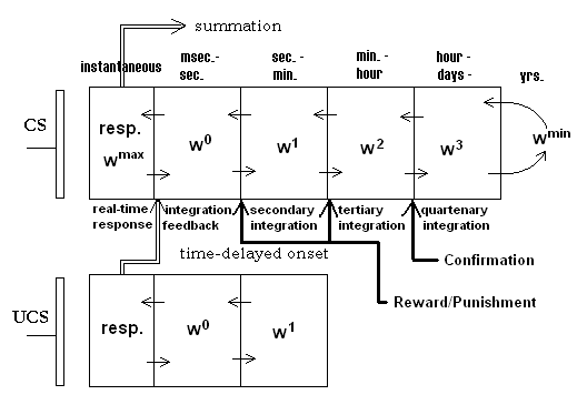
Figure 2. An adaptrode model showing multiple time domains in the adaptrode filter.

The details of adaptrode equations have been given elsewhere more extensively[17, 27 (Toward a Theory of Learning and Representing Causal Relations in Neural Networks)]. Here we present a summary of the relevant difference equations to motivate the above figures. In these equations (t) denotes a discrete time step. With a high sample rate, equivalent to the maximum action potential rate of a neuron (around 100 - 200/sec.), the dynamical properties of the adaptrode closely approximate those of real synapses. Even with somewhat lower sample rates (10/sec) we have found that the weight trajectories still follow reasonably close to those synapses. At high rates the input value, x0(t) below, is simply set to 1 to represent an action potential or 0 for none, thus emulating a spiking neuron. At lower rates we use a time-averaged fraction of the maximum input value between 0 and 1.

In what follows note that the use of superscripts to index the time domains or levels in an adaptrode. Subscript indexes have been used to specify neuron and adaptrode number in a matrix but are omitted here. The superscripted index is used for historical consistency.

The response (resp. in the figure) of an adaptrode is the result of the input signal and is used in the summation process (below). It is given by:

where:

     r(t+1) = response at next time step
     r(t) = response at current time step
     w⁰(t) = zeroth level synaptic weight at current time step
     x⁰(t) = zeroth level input to the synapse — the primary axonal input
     δ^r = decay constant for response, 0 ≤ δ^r ≤ 1

The response decays at an independent rate from that of the first level weight so that during periods of quiescence the adaptrode produces no significant output.

The value of w^l(t), the weight at level l, is given by:

where:

l = {0, 1, 2,...L} is an index of the adaptrode level
x⁰ = {0, 1}
w^l-1 = w^max for l = 0
w^l+1 = w^min for l = L

α, δ = (0, 1) are rate constants. Generally, α^l < α^l-1 and δ^l << δ^l-1
Δt is some number of time steps, dependent on the rate constants used.

Note that Eq. 2a establishes the time-ordering conditions under which the level 1 weight is increased.

Eq. 2 may be applied recursively by level, starting with l = 0. The value of w^max need not be a constant but in the simple, linear case, it is set to 1. A nonlinear case allows for w^max to start at a low value and increase as a function of w^L. This case is interesting for modeling dendritic spines but is not discussed further here.

Equation 2 can be derived rather straightforwardly from the exponential smoothing function (leaky integrator). Several researchers have used this function to represent memory traces in simulations of neural processing. Given some α between 0 and 1 that function is given by:

rearranging terms and substituting the exponential decay constant with a smaller decay constant, δ:

where δ <<: α

Since we have decoupled the decay from the increase it is necessary to introduce a simple shunting term to prevent w from exceeding some desired maximum, 1 in this case:

where w^max can be set to 1, thus keeping w within the range 0,1.

Using the same strategy for shunting the decay term so that w never falls below some lower limit, and, introducing the level index, l, letting that limit be the wl+1 value of a second level in which the increase and decay constants are less than the higher level, we create a multi-staged smoothing filter. As will be seen in comparing the graphs of equations 2 (Graph 1) and 3 (Graph 2), simple exponential smoothing is problematic in providing a real memory trace mechanism. Not shown in Graph 1 is the fact that the traces will continue to decay at the d2 rate. However, the value of w0 is maintained at some elevated level. Thus, when another pulse arrives at the synapse, its response will start from an elevated value. The EWA method quickly returns to zero (asymptotically close) and therefore cannot represent a longer-term memory trace.

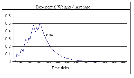
Graph 1. Trace of an exponential weighted average (smoothing), equation (3). The spikes in the trace indicate where an input spike at x⁰ occurred. Note the fast exponential falloff after offset of the input signal. Note also that while the shape is similar to that in Graph 2, below, the maximum value of the ewa is more than 0.2 less than w⁰. α = 0.1. Input data was the same as in Graph 2.

The input variable x^l for level 1 of the adaptrode in Figure 2 results from the response of a nearby non-associative adaptrode, but is gated by the time of arrival of spike episodes (Eq. 2a). If a spike episode arrives at the UCS adaptrode before one arrives at the CS adaptrode, then the x¹ signal is kept to 0, thus preventing potentiation in Eq. 2 at l = 1. x¹ for l < 1 are simply response signals, time averaged, from neurons used to represent reward/punishment and confirmation sources (to be described below). For example, at level 2, if a reward neuron (say one detecting the touch of a specific resource object) is not activated when the adaptrode is potentiated at w¹, then the potentiation of w² will be blocked resulting in no rise in w². Subsequently, over time, w¹ will decay further than it would have had the reward neuron been active. Conversely, had the reward neuron been active, w² would be potentiated leading to a slower decay in w¹ (see graph below).

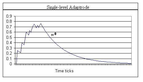
Graph 2. A single level adaptrode shows the effect of decoupling the decay from the increase of a memory trace mechanism. Note the longer time over which a memory trace lasts as compared to that in Graph 1. α⁰ = 0.25, δ⁰ = 0.05.

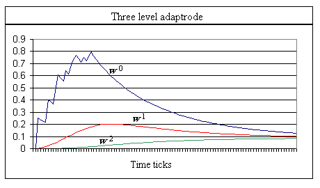
Graph 3. The traces of w⁰, w¹ and w² of a three-level adaptrode are shown with the same input data. This adaptrode is non-associative; the gating between each level is set to 1.0. Note the extended trace of w⁰ buoyed by the lower levels. α⁰ = 0.25, δ⁰ = 0.05, α¹ =0.03, δ¹ = 0.07, α² = 0.01, δ² = 0.0001. Values were set to capture the essential shapes in a graph.

The trace of w⁰ in Graph 3 has the same qualitative features as seen in long-term potentiation in biological synapses; it has a similar temporal integration trajectory. In the context of artificial neurons, the adaptrode has been shown to allow the construction of very simple neural networks that accomplish what would otherwise require complex and elaborate networks of conventional neurons. Simply stated, it would require multiple recurrent loops of varying lengths of neurons to provide the memory and time delay features of the a single adaptrode.

As can be inferred from Graph 3, subsequent input episodes (spike bursts) result in faster, stronger responses from adaptrodes that have been potentiated. In a neuron, with spatial integration, following the scheme suggested in Figure 2, the adaptrode acts to capture temporally ordered correlations over multiple time scales. When sufficiently potentiated, the CS adaptrode can generate a neuronal output on its own. Thus the CS signal becomes a reliable predictor of the UCS by eliciting a conditioned response, anticipating the onset of the UCS itself.

A typical associator neuron is shown in Figure 3 below. This neuron is used to associate one (or more) of a set of different CS signals with a single, semantically relevant UCS signal. The association is acquired by on-going experience, given appropriate reward and confirmation feedback. Eventually a correlated CS signal can activate the neuron by itself when the adaptrode is sufficiently potentiated. This neuron acts as an anticipator — the onset of a CS alone can elicit a response that produces a behavior appropriate for handling the cause of the UCS even before the onset of the UCS. Such an anticipation capability has obvious biological and evolutionary benefit.

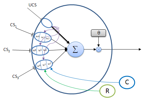
Figure 3. A typical neuron with adaptrode inputs (ovals). The UCS input, represented by a single line terminus, produces a strong response (thick black arrow to the summation and purple arrows to each associative adaptrode) which generally exceeds the threshold value, θ, thus causing the neuron to output a spike (or train of spikes). The various input responses from all adaptrodes are summed (Σ). Ordinarily, CS input responses would not be sufficient to fire the cell. If one of the CS inputs signals is highly correlated (with appropriate time delay) with the UCS, and has been rewarded and confirmed by past experience, then its response could exceed θ and result in an output from the neuron. Only reward (R, green circle that gates the w¹ level) and confirmation (C, blue circle that gates the w² level) signals reaching CS3 adaptrode are shown to prevent clutter, however these signals reach all of the CS adaptrodes. The response from the UCS adaptrode is used for the level 1 gate (purple arrows) to the CS adaptrodes.

5. A Robot Control Architecture, Behavior and the Ecology

MAVRIC (Mobile Autonomous Vehicle for Research in Intelligent Control) is a robot used to investigate adaptive behavior[28, 29, 31 (MAVRIC's Brain)]. Implemented with an augmented ActivMedia Pioneer I platform, MAVRIC uses an Extended Braitenberg Architecture[4, 32] based on adaptrode neurons. Its sensory capabilities have been extended to include four semi-directional light sensors, four tone detectors simulating odorant detection and two aural detectors (four tones each) for a total of 16 additional analog inputs. Two of the odorant tones have been predesignated as “physiologically meaningful” stimuli, food and poison. These are used as unconditioned stimuli that initiate trophic behaviors (attraction/seeking or aversion). The robot is equipped with seven sonar range finders, shaft encoders and bump detectors. In order to obtain the additional analog I/O it was necessary to abandoned the front gripper. However, since the objective of our research is demonstrating the learning of environmental contingencies rather than manipulation tasks, this has not proven to be problematic.

MAVRIC’s brain is comprised of a neural network employing both simple reactive neurons and more complex associative adaptive neurons using adaptrode-based synapses. The brain is comprised of a perceptual processing layer receiving inputs from the sensors and producing feature/object information, an associative processing layer for learning causal relations between features and objects, and a motor control layer. Each of these, in turn is composed of several sub-layers responsible for specialized processing. For example, the perceptual layer includes sub-layers for reaction to unconditioned stimuli such as a “food” tone or a “poison” tone, a sub-layer for orienting object locations relative to the agent’s centerline, and a general sub-layer for detecting specific features such as light intensity, odor (tone) gradients, etc.

The motor control layer is a good example of an attempt to mimic biological systems more closely. The core of this layer is comprised of a central pattern generator (CPG) oscillator circuit described more extensively in Mobus[29, 31]. In typical robot implementations that involve a wander behavior (for exploring the environment) this is accomplished by a random walk process. Animals, however, do not exhibit random walk properties in their locomotion (see below). We have found that the use of this oscillator circuit produces a number of animal-like movement patterns useful in the task domain. Moreover, the transition from one kind of pattern to a different one is smooth, allowing apparent mixtures of pattern. Originally this circuit was implemented using adaptrode neurons to obtain the desired dynamics. More recently we have found a simpler simulation that allows us to reduce the biological realism, thus increasing the computational speed, without sacrificing the behavior performance. This finding lends support to the notion that there may be optimal degrees of biomimicry at any given level.

Learning associations as the basis for behavior modification is at the heart of MAVRIC’s brain. Figure 4 depicts a simple associator network comprised of two cells. The objective of this network is to learn which combinations of features portend a resource (food) or a threat (poison). There are two behaviors that derive from this network; seeking (food) and avoidance (poison). The cell architecture is the same as in Figure 3. An unconditioned stimulus (food/poison) gates the potentiation of adaptrode synapses (conditioned stimuli) receiving inputs from the perceptual layer. Rewards/punishments and confirmation signals come from internal state sensors in the robot. The output of this layer goes to the motor control layer where decisions about which direction to turn are made depending on whether the object is on the left, right or in front and whether the action should be to avoid or seek. Inputs at either food or poison unconditionally generate appropriate output signals. Avoidance will inhibit seeking. Once this circuit has formed associations between the various feature combinations and the unconditioned stimulus, input of only those features will activate the appropriate associator neuron. Note that, prior to any learning the circuit is wired so that any combination is learnable. Only those combinations that causally associate with the respective UCS will lead to potentiation of the corresponding adaptrode, and hence generate activity in the neuron. The non-potentiated adaptrodes remain present and able to capture any changes, short- or long-term, in the associative combintations.

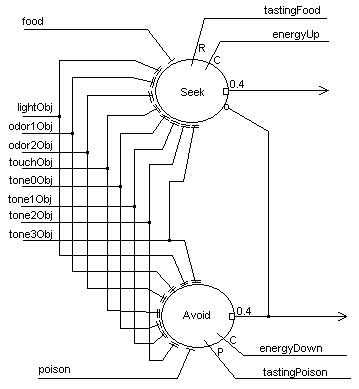
Figure 4. The associator network for an autonomous agent.

Destructive interference refers to the phenomenon where two or more patterns interfere with each other when adjusting the weights in a connectionist, particularly supervised, learning system. This arises where all link weights are governed by the same learning rate constant. It is essentially the same phenomenon that causes such networks to learn very slowly. They must search a substantial portion of weight space to find those zones where the patterns to be learned do not compete for setting weight values.

Continuous learning as implemented in self-supervising and unsupervised learning systems also suffers from destructive interference. Such learning is needed to address the issue of nonstationarity in the environment. Consider the following scenario. A robot learns that a bright light represents a power supply. The causal association between light and power is established over a long time scale through consistent reinforcement. It will routinely approach such a cue when it needs power replenishment. What happens if the world changes? Suppose that fire is introduced into the world. It produces a bright light that the robot is drawn toward. But instead of reward the robot (assuming it can detect heat) gets a punishment. What should it learn? The two conditions are contrary. If the robot uses a single time-domain learning mechanism, it will be forced to learn an association between punishment and light to the detriment of the earlier association. This phenomenon is most pronounced in algorithms for fast continuous learning where recency effects amplify the problem.

As discussed in the section above, on dynamic synapses, the multi-time domain model of synaptic processing provides a means to retain a long-term memory trace, called savings, even while forming short-term contrary memories. In a network such as in Figure 4 it is possible to have a long-term memory trace encoded in the “lightObj” adaptrode through the Seek neuron. A short-term trace could be encoded in the “lightObj” adaptrode of the Avoid neuron representing the recent change in association between light and punishment. Such a trace, in the w0 value, would be stronger than the long-term trace in the Seek neuron, but would also tend to decay more rapidly. Hence, the agent can have both memories encoded, one in short-term form, the other in long-term form, without conflict between them. If after a time the situation returns to “normal”, i.e., the long-term relation between light and power is re-established, then the short-term trace will decay rapidly leaving the long-term trace intact (c.f. [27]).

6. Foraging for Resources in an Open, Nonstationary World

The task set before MAVRIC is to forage for sparsely distributed resources (food) in a vast, open and nonstationary world while avoiding danger[31, 33 (Foraging Search: Prototypical Intelligence)]. It must successfully find resources within time constraints to replenish an internal energy reservoir. Foraging, as used here, is substantially different from the foraging task often described for robot research[3, 4, 34]. The latter, perhaps better described as a gathering task, is often conducted in a closed world, usually small relative to the sensory range of the robots, where sought items may be densely distributed. Generally, the sought items (e.g., soda cans) have stationary characteristics, though some researchers have examined the effects of nonstationary conditions within the task environment.

Foraging in animals actually involves a number of complex sub-tasks, of which handling (consuming or gathering) is but one[35-44]. But primarily it is a problem in finding a resource. Typically resources (like food, water, shelter) are sparsely distributed over a large territory relative to the size of the animal. Furthermore, resources are distributed in stochastic, but not random, patterns. There is some evidence to suggest that distributions are governed by 1/f or chaotic dynamics. Food, for example, often is found in patches (vegetation or population concentrations of prey) of varying size and quality and the distance between patches along a transect of the territory is highly variable owing to variations in the topology and substrates of the area. Added to this are seasonal factors and competition from other species. All of which makes it impossible to learn a fixed pattern of resource availability.

Studies of foraging behavior strongly suggest that animals, even very simple ones, find resources by learning contingent cues that are causally linked to the resource. To be useful cues must be detectable from a greater distance than direct detection of the resource itself, and the causal relation must be sufficiently reliable. Visual detection of flower shape by foraging bees is an example of such a cue. Bees learn which flowers are producing higher quality nectar and use the shape to guide further foraging effort. Flowers may undergo variations in their nectar production, in multiple time scales, so bees need to be able to learn quickly which species are currently producing the highest quality nectar to optimize their foraging effort.

The general framework for foraging is composed of two behaviors that form poles on a continuum. Activities associated with either pole can transition smoothly from one end to the other. The first behavior, in which the animal either detects no cues or is naïve about cue-resource relations, is marked by a characteristic search pattern. In most species this is clearly not a pure random walk search. Nor is it a systematic search, such as a widening spiral or move in a straight line. Rather, the animal wanders in a drunken sailor walk (produced by the CPG oscillator discussed above). The path is novel, but not random. Elsewhere we have discussed the advantages of this pattern for naïve search. The pattern is more likely to bring the animal into contact with a resource in a timely fashion than either random or systematic search.

If the animal is naïve it needs to learn the surrounding context of the occurrence of a resource that might provide relevant cues. In the case of the bee, it forms a short-term memory of the flower shape features upon which it has alighted (bees are drawn to generalized flower shapes). If, subsequently, the flower produces a high reward payoff, the short-term memory is retained in an intermediate form. The bee can then test other similar flowers for confirmation of the reward (Waddington & Heinrich). Thus the animal extracts a causal cue-resource relation from its experience. What is critical here is that the cue must be perceived before the resource is detected otherwise it has no value as a cue.

A more directed motion marks the second behavior. Once a previously learned cue is detected the animal orients its motion on the cue and follows whatever gradient information it obtains to approach the cue as if it were detecting the resource itself. The cue need only be within a proximity to the actual resource such that the animal is brought into detection range of the latter. The attraction to the resource can then supercede the attraction to the cue allowing the animal to home in on the former. Thus in the presence of a learned cue the animal can efficiently find the resource.

In our experimental setup MAVRIC operates in a gymnasium where resource/threat objects can be distributed so that their sensible features can initially lie far beyond the range of the robot sensors. Additionally the resources can be spread out such that the robot could easily find a transect that would allow it to traverse the territory without detecting them. That is, the resources are sparsely distributed. MAVRIC’s task then, is to search for sparse resources in a completely uncertain world.

The experimental situation is made even more realistic by having no actual boundaries. The work area for the robot is a large square area, monitored from above by a remote TV camera and a frame grabber in a “world” computer. When the robot roams, if it crosses over the line it is paused at that point. The computer generates the environment in a square area adjacent to the crossing point. The old environment (objects placed in the working area) is removed and the new environment is set up in the old area. The robot is then moved to the contra-lateral position as if just coming into the environment. Then the robot is re-activated and the run continues. In this way we are able to effectively simulate an open world. There is no limit on the number of environment plans that can be generated.

The objects in this framework are portable, battery powered sensate sources (tones and lights) that operate under radio control. Each object is uniquely addressed and is controlled by the “world” computer. As the robot approaches or moves away from each object, the computer can raise or lower the intensity of the sensate, thus simulating a gradient. MAVRIC’s brain includes an olfactory simulation (using tones) and can follow an odorant gradient (up or down).

7. Discussion

The presented model is by no means an attempt to simulate every detail of real biological synapses. Indeed, it only addresses post-synaptic processes. There are a wide variety of pre-synaptic contributions to learning. This model should not be thought of as a model of biological processes. Rather, it attempts to capture the essence of the dynamic properties of synapses, specifically the cumulative effects on membrane potential. Accordingly we are only claiming that it is a more deeply inspired model than classical ANNs. The question we open in this paper is: What benefit might derive from greater biomimicry in neural processing?

Clearly, biological synapses perform significant processing in the encoding of temporally ordered signals whose relations extend over significant time scales. The model has deep implications for the kinds of problems that biological systems solve in learning, memory and cognitive phenomena. We mention a few here.

Destructive interference problem: As discussed above.

Symbol-grounding problem[45]: If “symbol” is interpreted as a specific neural representation then the CS-UCS association learning addresses the issue of learning biologically relevant correlations, or in other words, giving “meaning” to otherwise neutral stimuli. Damasio[46] has suggested a neurological framework in which higher-order representations are grounded in biological meaning to an organism through experientially acquired valence dispositions. Associative neurons, such as above, have the capacity to encode such dispositions. As MAVRIC forages it is able to continually learn those associations between cue objects and resource objects. Cues are defined as objects that are causally related to the resource. The resource is, by definition, meaningful to the robot. Cues come to have meaning by virtue of their causal relation and the robot’s ability to learn that relation.

Frame problem[47]: Of all the possible stimuli to which an agent could attend, which ones should it attend? Valence dispositions acquired through an associative network as in Figure 4 suggest a solution to this problem. An agent is actually perceptive, at a low level, to all salient stimuli. Of these, only a few will actually contribute to receiving reward or punishment and, hence become associated with relevant action through potentiation. Over time, the most predictive stimuli will persist. Periodic pruning of non-potentiated adaptrodes could simplify the network and the computation load. We intend to test this in the MAVRIC robot by increasing the number of non-relevant objects (and their feature sets) in the environment. MAVRIC will then have many more stimuli to choose from in selecting relevant cues.

Credit assignment problem[48-51]: The solution of this problem in reinforcement and value-based learning has been extensively covered in the literature. The adaptrode approach simply extends these arguments to multiple time scales (see also [52]).

8. Conclusion

We have argued that greater biological fidelity may pay off in more realistic biological-like behavior, but only if that fidelity is justified across levels of organization. Here we have presented a more biomimic neural processor/learning mechanism and related it to both the nervous system level and behavioral/ecological levels in an autonomous agent. The latter level represents a more complete test of autonomy. The middle level connects the competencies of the neural level with the demands of the behavior level. The foraging search task as described here is more extensive than the gathering task generally cited in the literature. The accomplishment of such an extensive task is enabled by the ability to learn associations on a variety of time scales as implemented in the adaptrode mechanism.

9. Acknowledgements

The research reported here is funded in part by a grant from the College of Arts & Sciences, Western Washington University and by National Science Foundation grant IIS-9907102. We are grateful to Paul Fisher for his early support of research on the adaptrode and its application to robotics.

10. References

1. Meyer, J.-A. and A. Guillot. “Simulation of adaptive behavior in animats: Review and prospect”. in First International Conference on Simulation of Adaptive Behavior: From Animals to Animats. 1991: The MIT Press.
2. Alkon, D.L., et al., “Pattern Recognition by an Artificial Network Derived from Biological Neuronal Systems”. Biological Cybernetics, 1990. 62: p. 363-376.
3. Arkin, R.C., Behavior-Based Robotics. 1998, Cambridge, MA: The MIT Press.
4. Pfeifer, R. and C. Scheier, Understanding Intelligence. 1999, Cambridge, MA: The MIT Press. 697.
5. Grossberg, S., “A Neural Network Architecture for Pavlovian Conditioning: Reinforcement, Attention, Forgetting, Timing”, in Neural Network Models of Conditioning and Action, M.L. Commons, S. Grossberg, and J.E.R. Staddon, Editors. 1991, Lawrence Erlbaum Associates, Publishers: Hillsdale, NJ. p. 69-122.
6. Carpenter, G.A. and S. Grossberg, “A Massively Parrallel Architecture for a Self-organizing Neural Pattern Recognition Machine”. Computer Vision, Graphics, and Image Processing, 1987. 37: p. 54-115.
7. Carpenter, G.A., “Neural Network Models for Pattern Recognition and Associative Memory”. Neural Networks, 1989. 2: p. 243-257.
8. Carpenter, G.A., S. Grossberg, and J.H. Reynolds, “ARTMAP: Supervised Real-time Learning and Classification of Nonstationary Data by Self-organizing Neural Networks”. Neural Networks, 1991. 4(5): p. 565-588.
9. Crick, F., “The recent excitement about neural networks”. Nature, 1989. 337: p. 129-32.
10. Rumelhart, D.E. and J.L. McClelland, Parallel Distributed Processing: Explorations in the Microstructure of Cognition, Vol. 1: Foundations. Parallel Distributed Processing: Explorations in the Microstructure of Cognition, ed. D.E. Rumelhart and J.L. McClelland. Vol. 1. 1986, Cambridge, MA: The MIT Press.
11. Rumelhart, D.E. and J.L. McClelland, Parallel Distributed Processing: Explorations in the Microstructure of Cognition, Vol. 2: Psychological and Biological Models. Parallel Distributed Processing: Explorations in the Microstructure of Cognition, ed. D.E. Rumelhart and J.L. McClelland. Vol. 2. 1986, Cambridge, MA: The MIT Press.
12. Michaud, F. and M.J. Mataric, “Learning from History for Behavior-Based Mobile Robots in Non-stationary Conditions”. Machine Learning, 1998. 31(1-3): p. 141-167.
13. Mataric, M.J., “Great Expectations: Scaling Up Learning by Embracing Biology and Complexity”. 1998, University of Southern California, NSF Workshop on Knowledge Models and Cognitive Systems.
14. Alkon, D.L., Memory Traces in the Brain. 1987, Cambridge, MA: Cambridge University Press.
15. Alkon, D.L., et al., “Memory Function in Neural and Artificial Networks”, in Neural Network Models of Conditioning and Action, M.L. Commons, S. Grossberg, and J.E.R. Staddon, Editors. 1991, Lawrence Erlbaum Associates, Publishers: Hillsdale, NJ. p. 1-11.
16. Mackintosh, N.J., Conditioning and Associative Learning. 1983, London: Oxford University Press.
17. Mobus, G.E., A Multi-time Scale Learning Mechanism for Neuromimic Processing, Unpublished dissertation in Computer Science. 1994, University of North Texas: Denton. p. 127.
18. Pavlov, I.L., Conditioned Reflexes. 1927, London: Oxford University Press.
19. Hebb, D.O., The Organization of Behavior. 1949, New York: Wiley.
20. Baxter, D.A., et al., “Empirically Derived Adaptive Elements and Networks Simulate Associtative Learning”, in Neural Network Models of Conditioning and Action, M.L. Commons, S. Grossberg, and J.E.R. Staddon, Editors. 1991, Lawrence Erlbaum Associates, Publishers: Hillsdale, NJ. p. 13-52.
21. Byrne, J.H. and K.J. Gingrich, “Mathematical model of cellular and molecular processes contributing to associative and nonassociative learning in Aplysia”, in Neural Models of Plasticity, J.H. Byrne and W.O. Berry, Editors. 1989, Academic Press: Orlando, FL. p. 58-72.
22. Jaffe, D. and D. Johnston, “Induction of long-term potentiation at hippocampal mossy-fiber synapses follows a Hebbian rule”. Journal of Neurophysiology, 1990. 64: p. 948-960.
23. Sejnowski, T.J., S. Chattarji, and P. Stanton, “Induction of synaptic plasticity by Hebbian covariance in the hippocampus”, in The Computing Neuron, R. Durbin, C. Miall, and G. Mitchison, Editors. 1989, Addison-Wesley: Reading, MA. p. 105-124.
24. Small, S.A., E.R. Kandel, and R.D. Hawkins, “Activity-dependent enhancement of presynaptic inhibition in Aplysia sensory neurons”. Science, 1989. 243: p. 1603-1605.
25. Staddon, J.E.R., “On Rate-Sensitive Habituation”. Adaptive Behavior, 1993. 1(4): p. 421-436.
26. Starmer, C.F. “Characterizing synaptic plasticity with an activity dependent model”. in IEEE First International Conference on Neural Networks. 1987. San Diego, CA: Institute for Electrical and Electronic Engineers.
27. Mobus, G.E., “Toward a Theory of Learning and Representing Causal Inferences in Neural Networks”, in Neural Networks for Knowledge Representation and Inference, D.S.Levine and M. Aparicio, Editor. 1994, Lawerence Erlbaum Associates: Hillsdale, NJ. p. 339-374.
28. Mobus, G.E. and P.S. Fisher, “A Mobile Autonomous Robot for Research in Intelligent Control”. 1993, Center for Research in Parallel and Distributed Computing, University of North Texas: Denton, TX.
29. Mobus, G.E. and P.S. Fisher. “MAVRIC's Brain”. in International Conference on Industrial and Engineering Applications of Artificial Intelligence and Expert Systems (IEA-AIE). 1994. Austin, TX.
30. Mobus, G.E. and M. Aparicio. “Foraging for Information Resources in Cyberspace: Intelligent Foraging Agent in a Distributed Network”. in Center for Advanced Studies Conference, CASCON'94. 1994. IBM, Toronto.
31. Mobus, G.E. and P.S. Fisher, “Foraging Search at the Edge of Chaos”, in Oscillations in Neural Systems, D.S. Levine, V.R. Brown, and V.T. Shirey, Editors. 2000, Lawerence Erlbaum Associates: Mahwah, NJ. p. 309-326.
32. Braitenberg, V., Vehicles: Experiments in Synthetic Psychology. 1984, Cambridge, MA: The MIT Press.
33. Mobus, G.E. Foraging Search: “Prototypical Intelligence”. in Computing Anticipatory Systems, CASYS'99. 1999. Liège, Belgium: American Institute of Physics.
34. Arkin, R.C., “Behavior-Based Robot Navigation for Extended Domains”. Adaptive Behavior, 1992. 1(2): p. 201-225.
35. Collier, G.H. and C.K. Rovee-Collier, “A comparative analysis of optimal foraging behavior: laboratroy simulations”, in Foraging Behavior, A.C. Kamil and T.D. Sargent, Editors. 1981, Garland STPM Press: New York. p. 39-76.
36. Dow, S.M. and S.E.G. Lea, “Foraging in a changing environment: simulations in the operant laboratory”, in Quantitative Analysis of Behavior: Foraging, M.L. Commons, A. Kacelnik, and S.J. Shettleworth, Editors. 1987, Lawerence Erlbaum Associates: Hillsdale, NJ. p. 89-114.
37. Garber, P.A. and B. Hannon, “Modeling monkeys: a comparison of computer-generated and naturally occurring foraging patterns in two species of neotropical primates”. International Journal of Primatology, 1993. 14: p. 827-852.
38. Kacelnic, A., J.R. Krebs, and B. Ens, “Foraging in a changing environment: an experiment with starlings (Sturnus vulgaris)”, in Quantitative Analysis of Behavior: Foraging, M.L. Commons, A. Kacelnik, and S.J. Shettleworth, Editors. 1987, Lawerence Erlbaum Associates: Hillsdale, NJ. p. 63-88.
39. Kristan, W., et al., “Behavioral choice - in theory and in practice”, in The Computing Neuron, R. Durbin, C. Miall, and G. Mitchison, Editors. 1989, Addison--Wesley Publishing Co.: New York. p. 180-204.
40. Menzel, E.W. and E.J. Wyers, “Cognitive aspects of foraging behavior”, in Foraging Behavior, A.C. Kamil and T.D. Sargent, Editors. 1981, Garland STPM Press: New York. p. 355-377.
41. Milton, K., “Foraging behavior and the evolution of primate intelligence”, in Machiavellian Intelligence: Social Expertise and the Evolution of Intellect in Monkeys, Apes, and Humans, R. Byrne and A. Whiten, Editors. 1988, Oxford University Press.
42. Rashotte, M.E., J.M. O'Connel, and V.J. Djuric, “Mechanisms of signal-controlled foraging behavior”, in Quantitative Analysis of Behavior: Foraging, M.L. Commons, A. Kacelnik, and S.J. Shettleworth, Editors. 1987, Lawerence Erlbaum Associates: Hillsdale, NJ. p. 153-179.
43. Shettleworth, S.J., “Learning and foraging in pigeons: effects of handling time and changing food availabiltiy on patch choice”, in Quantitative Analysis of Behavior: Foraging, M.L. Commons, A. Kacelnik, and S.J. Shettleworth, Editors. 1987, Lawerence Erlbaum Associates: Hillsdale, NJ. p. 115-132.
44. Waddington, K.D. and B. Heinrich, “Patterns of movement and floral choice by foraging bees”, in Foraging Behavior, A.C. Kamil and T.D. Sargent, Editors. 1981, Garland STPM Press: New York. p. 215-230.
45. Harnad, S., “The Symbol Grounding Problem”. Physica D, 1990. 42: p. 335-346.
46. Damasio, A.R., Descarte's Error: Emotion, Reason and the Human Brain. 1994, New York: G. P. Putnam's Sons. 312.
47. McCarthy, J. and P.J. Hayes, “Some philosophical problems from the standpoint of artificial intelligence”. Machine Intelligence, 1969. 4: p. 463-502.
48. Staddon, J.E.R. and Y. Zhang, “On the Assignment-of-Credit Problem in Operant Learning”, in Neural Network Models of Conditioning and Action, M.L. Commons, S. Grossberg, and J.E.R. Staddon, Editors. 1991, Lawrence Erlbaum Associates, Publishers: Hillsdale, NJ. p. 279-293.
49. Sutton, R.S. and A.G. Barto, “Toward a Modern Theory of Adaptive Networks: Expectation and Prediction”. Psychological Review, 1981. 88: p. 135-171.
50. Sutton, R.S., “Learning to predict by the methods of temporal difference”. Machine Learning, 1988. 3: p. 9-44.
51. Sutton, R.S. and A.G. Barto, “Time-Derivative Models of Pavlovian Reinforcement”, in Learning and Computational Neuroscience: Foundations of Adaptive Networks, M. Gabriel and J. Moore, Editors. 1990, The MIT Press: Cambridge, MA.
52. Sutton, R.S. “TD Models: Modeling the World at a Mixture of Time Scales”. in Proceedings of the 12th International Conference on Machine Learning. 1995.