Particle methods

Many scientific problems can be tackled using particle methods, in which a large collection of discrete particles are individually tracked as they move relative to one another. Often the motion is governed by laws of physics such as Newton’s law force = mass times acceleration, which determines the acceleration of each particle from the forces acting on it, which in turn might depend on the location of all the particles. This leads to differential equations to solve for the locations (since acceleration is the second derivative of location).

If the particles are indexed by j = 1, 2, \ldots, N for some (often very large) number of particles N, and the locations and velocities at time t are denoted by x_j(t), y_j(t), z_j(t) and u_j(t), v_j(t), w_j(t) respectively, then the differential equations we need to solve are:

x_j'(t) = u_j(t), \quad u_j'(t) = F_{1j}(x(t),y(t),z(t)),

y_j'(t) = v_j(t), \quad v_j'(t) = F_{2j}(x(t),y(t),z(t)),

z_j'(t) = w_j(t), \quad w_j'(t) = F_{3j}(x(t),y(t),z(t)),

where, for example, F_{1j}(x,y,z), is the x-component of the force acting on particle j based on the location of all other particles.

We will look at variations of this problem as model problems in this course, starting with a much simpler case where particles are moving only in the x-y plane and the velocities are specified rather than determined by solving a differential equations. See Rotating particles and Python efficiency.

Particle methods generate nice test problems for high performance computing since they can be very easy to formulate with minimal mathematics and yet be made arbitrary large and hard to solve by increasing the number of particles.

Note that very sophisticated mathematical and algorithmic ideas must often be used to efficiently solve these problems for large N, particularly when the force on each particle depends on the location of all other particles (the N-body problem). Since computing the force for each particle seems to require O(N) work and there are N particles, moving all particles may take O(N^2) work each time step, and one may need to take millions of time steps. There are algorithms such as tree-based codes and fast multipole methods that can drastically reduce the computing time required, but we will not be able to get into these in this course.

Below are a few applications of particle methods with pointers to some images and information about the calculations to give a flavor of large scale scientific computing in action.

Rotating particles

This is simple example is used for comparing the efficiency of various ways of writing a simple computer program in the sections Rotating particles and Python efficiency and Rotating particles and Fortran efficiency.

A set of particles in 2 space dimensions (the x-y plane) are initialized and then moved around. Here the motion is simply taken to be rotation about the origin.

To initialize the particles we will simply take N points along some parameterized curve:

x_j = 2. + r(\alpha_j)\cos(\alpha_j)

y_j = r(\alpha_j)\sin(\alpha_j)

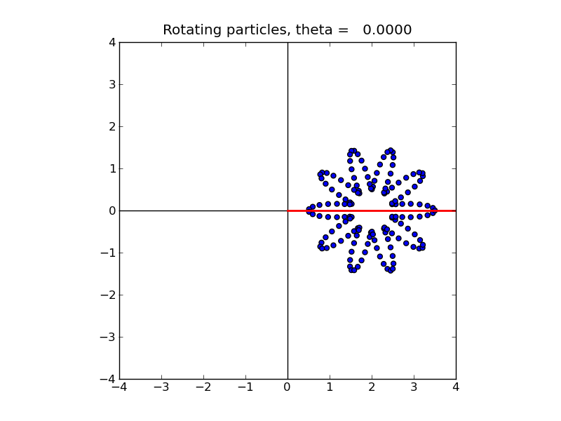
for 0 \leq \alpha \leq 2\pi. The radius function r(\alpha) defines a radius that can vary with \alpha. If r(\alpha)\equiv 1 for all \alpha then the particles would lie on a circle of radius 1 centered at (2,0). Here we use r(\alpha) = 1.0 + 0.5\cos(10\alpha) just to give a more interesting curve.

With 150 particles, they are initially located as in this figure:

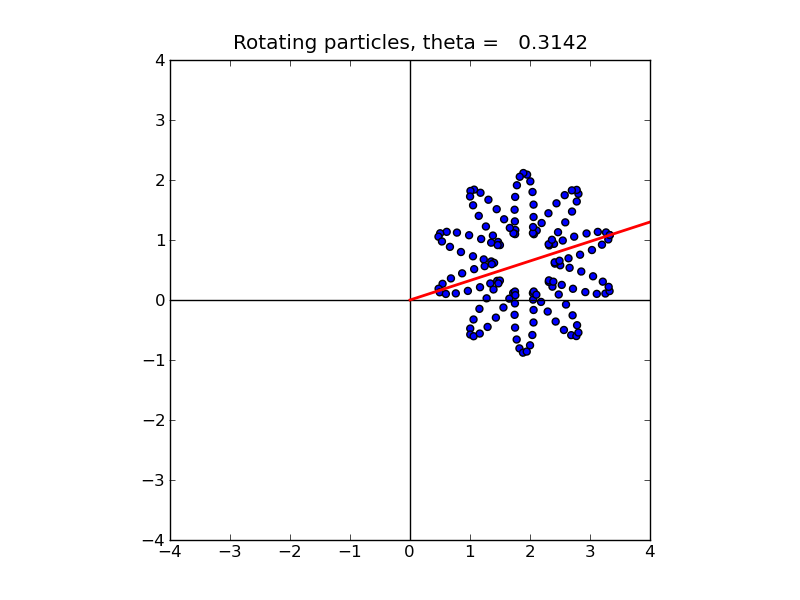
We now rotate these particles about the origin. In the code below, theta refers to the rotation angle \theta, which varies from 0 to 2\pi. For example, with \theta = \pi/10 \approx 0.3142 the particles look like this:

Here the red line is for reference and shows the angle. [animation]

Cosmology

One application is to the study of galaxy formation and other large scale cosmological structures, in which case the particles may be individual stars or smaller units of matter. This problem is being studied in the N-Body Shop led by Tom Quinn in Astronomy at UW. See their image gallery for the results of some such simulations. As you’ll see from the captions, some of these calculations require millions or billions of particles and take hundreds of thousands of CPU hours to compute.

Granular flow and molecular dynamics

Particle methods are often used to model small scale physics problems too, such as the flow of granular materials (e.g. sand or grain in a hopper). At even smaller scales they are used to model individual molecules or even atoms within a molecule in materials science, molecular biology, and many other areas. A variety of results of this type can be found at the LAMMPS site. This stands for Large-scale Atomic/Molecular Massively Parallel Simulator, developed at Sania National Laboratory. See in particular their animations and benchmarks.

---

More applications to appear...