mmf.solve.solver_interface
| IProblem() | Interface for an iterative problem: the solver’s goal is to |
| IPlotProblem() | Generalization of IProblem that provide methods for |
| IState() | Interface for the state of a solution. |
| ISolver(state0) | Interface for solver objects. |
| ISolverData() | Interface for solver data objects. |
| IJinv() | Interface of a matrix-like object that represents the inverse |
| IMesg() | Interface to a messaging object. |
| IterationError | Iteration has failed for some reason. |
| Solver(*varargin, **kwargs) | Default partial implementation for solver objects. |
| SolverData(*varargin, **kwargs) | Default implementation of solver data objects. |
| Problem(*varargin, **kwargs) | Partial implementation of IProblem interface. Only state0 and one of G() or F() need2 to be defined (though both can be). |
| PlotProblem(*varargin, **kwargs) | Partial implementation of IPlotProblem interface. As with Problem, only G() and get_initial_state() need to be defined. |
| Problem_x(*varargin, **kwargs) | Partial implementation of IProblem interface. Same as Problem but with an additional attribute fn_rep representing a discretization. To be used with State_x, and provides an updated solver_update() utilizing this. |
| BareState(*varargin, **kwargs) | Default implementation of a bare IState. This only uses the flat representation of the state provided by x_. |
| State(*varargin, **kwargs) | Default implementation of IState with parameters. |
| State_x(*varargin, **kwargs) | Another default implementation of IState with parameters. This is the same as State except that it allows parameters with names that end with _x to be accessed or set as functions via the name without the _x using fn_rep – which must implement IFnRep – to convert between the two. |
| Mesg(*varargin, **kwargs) | Print the displayed messages immediately. |
| StatusMesg(*varargin, **kwargs) | This class acts like a message lists, but prints the current message in a status-bar without using up screen space. |
| solve(f, x0, solver[, store_history]) | Solve f(x) = 0 using specified solver and return the solution. |
| fixedpoint(f, x0, solver[, store_history]) | Solve f(x) = x using specified solver and return the solution. |
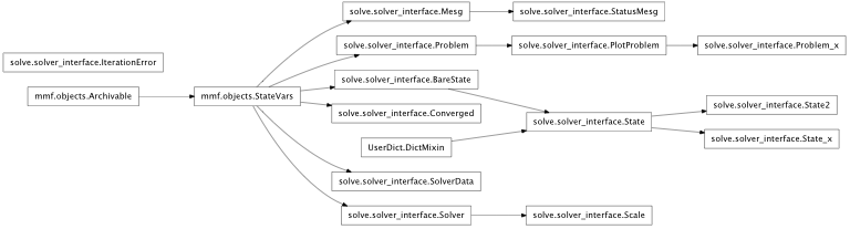
Inheritance diagram for mmf.solve.solver_interface:
This module contains the interface for solving root-finding and.or fixed-point problems of the forms:
0 == G(x)
x == F(x)
These can be related through the relationship F(x) = x - G(x), however, both forms have their use:
The 0 == G(x) form makes the objective function explicit and may be useful for specifying tolerances. One also may have an expression in terms of G for calculating a good step (for example, if the Jacobian can be calculated). Thus, the function Problem.G() returns a pair (G, dx) containing a suggested step (if it can be calculated).
This form also implicitly suggests that a good fixed-point iteration may not be known (which is why we always include a suggested step dx).
The x == F(x) form naturally suggests an iteration with dx = x - F(x) and so Problem.F() returns only the next step.
If present, this form is used to form the objective function G(x) = x - F(x) by memory-limited quasi-Newton methods such as the Broyden iteration which stores the inverse Jacobian as a matrix of the form B = I + D where D is rank deficient. The ideally convergent iteration F(x) = x_sol (always converging in a single step) would have
 , hence D = 0 and so this is
ideally captured by the rank deficient approximate Jacobian.
, hence D = 0 and so this is
ideally captured by the rank deficient approximate Jacobian.
These interfaces address the following functionality goals:
- Provide a history of the state of a solution so that the calculation can be reproduced.
- Allow for interaction with the solver, such as plotting/displaying intermediate results, prematurely terminating the solver, and possibly even adjusting the solution during the solution.
- Error recovery and reproduction.
The interface is defined by three main interfaces:
| IState | Interface for the state of a solution. |
| IProblem | Interface for an iterative problem: the solver’s goal is to |
| ISolver | Interface for solver objects. |
The general usage is something like:
problem = Problem(...)
solver = Solver(...)
state, niter = solver.solve(problem)
new_state, niter = solver.solve(problem, state)

# Archive
file = open(filename, 'w')
file.write(new_state.get_history())
file.close

...
# Restore
env = {}
execfile(filename, env)
state = env['state']
Problems and solvers are considered independent with the state information being stored in the return state object.
- IState
Specifies IState.x_, the current state of the solution. The abstraction employed here is that a state may be the result of three “transformations”:
- Initialization from a IProblem.get_initial_state() call.
- Initialization from direct assignment of x.
- Transformation from a previous state by a ISolver object.
The latter keeps track of the history of the state through the previous transformations/initializations so that the computation can be repeated.
- IProblem Specifies IProblem.initial_guess() which
implicitly defines the state class and problem size. A problem must implement the IProblem interface and specify at least one of the functions G(x) (to be set to zero) or F(x) (to find a fixed-point) by defining IProblem.step()
- state0 = IProblem.get_initial_state():
This provides the initial guess x0 which must implement the IState interface. This also defining the size of the problem so the solver can allocate resources etc.
(x1, G1, dx1, F1) = `:meth:`IProblem.step(): Returns the new step x1, the objective function G1 = G(x1), the suggested step dx1, and the fixed-point iteration F1=F(x1) based on the step x suggested by the solver. If the problem compute the Newton step dx1 = -np.dot(j_inv, G1) (as it will indicate by displaying IProblem.newton = True), then this should also be returned, otherwise, one should set dx1 = -G(x) as a default step.
The new step x1 need not be either of the natural steps x0 + dx or F1 allowing the problem more control, to enforce for example constraints or prevent the solver from wandering into unphysical regions of solution space.
- ISolver
- Provides a means for solving a problem. Once initialized, this provides a method to transform an initial guess (provided either by a Problem or by another State) into a new State.
Todo
Add and test support for a “global” dictionary used to allow the solver and problem to maintain state during the solution of a problem. Strictly, the calculation should not depend on this dictionary, but it can be used to store useful diagnostic information about the progress of the solution. Also, the dictionary can be used to maintain flags that control the iteration, thus allowing the user to alter or affect the iteration (from another process or thread). This use of a global dictionary has not been fleshed out yet but the idea is to allow one to use the mmf.async module for remote control.
To facilitate usage, partial implementations are provided:
States
| BareState(*varargin, **kwargs) | Default implementation of a bare IState. This only uses the flat representation of the state provided by x_. |
| State(*varargin, **kwargs) | Default implementation of IState with parameters. |
| State_x(*varargin, **kwargs) | Another default implementation of IState with parameters. This is the same as State except that it allows parameters with names that end with _x to be accessed or set as functions via the name without the _x using fn_rep – which must implement IFnRep – to convert between the two. |
Problems
| Problem(*varargin, **kwargs) | Partial implementation of IProblem interface. Only state0 and one of G() or F() need2 to be defined (though both can be). |
| PlotProblem(*varargin, **kwargs) | Partial implementation of IPlotProblem interface. As with Problem, only G() and get_initial_state() need to be defined. |
| Problem_x(*varargin, **kwargs) | Partial implementation of IProblem interface. Same as Problem but with an additional attribute fn_rep representing a discretization. To be used with State_x, and provides an updated solver_update() utilizing this. |
Solvers
| Solver(*varargin, **kwargs) | Default partial implementation for solver objects. |
As an example and to get started, look at the code for Scale and State2.
Tolerances
The general plan for determining if a parameter  is close enough to
 is to consider the condition err <= 1 where:
abs_err = abs(x - x_0)
rel_err = abs_err/(abs(x_0) + _TINY)
err = min(abs_err/(abs_tol + _TINY), rel_err/(rel_tol + _TINY))
This is True if either the absolute error is less than abs_tol or
the relative error is less than rel_tol. This is what we mean below
by  .
.
The real questions are:
What to use for
and ?There are two forms of solver here: Root finding
 and
fixed-point finding
and
fixed-point finding  . In general these are related by
 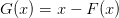 but some problems may define both. There is no
reference scale for
but some problems may define both. There is no
reference scale for  as it should be zero, so only the
absolute tolerance ISolver.G_tol makes sense here.
as it should be zero, so only the
absolute tolerance ISolver.G_tol makes sense here.It would be ideal if we could also provide a tolerance on the step
 , but this is only easy to implement with
bracketing algorithms. Instead, we may provide a heuristic based
on the Jacobian, but in general this is difficult to trust if the
Jacobian is not exact.
, but this is only easy to implement with
bracketing algorithms. Instead, we may provide a heuristic based
on the Jacobian, but in general this is difficult to trust if the
Jacobian is not exact.What to do when there is a vector of parameters?
The actual tolerance criterion used is:
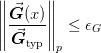
where the user can specify both the vector of typical scales
 through IProblem.G_scale and the
type of norm can be specified through ISolver.norm_p.
through IProblem.G_scale and the
type of norm can be specified through ISolver.norm_p.
Examples
Another way to use this is when representing functions in a discrete basis. In this case, one parametrizes the number of points used, and would like to be able to continue an iterative solution while increasing the resolution. Here is how it is done.
We will use as an example, the solution of the differential equation
 with boundary conditions
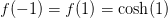 .
.
- interface mmf.solve.solver_interface.IProblem[source]
Bases: zope.interface.Interface
Interface for an iterative problem: the solver’s goal is to find a solution to the problem G(x) = 0.
The function G(), specified through step(), must accept a real vector x of the same dimension as returned by get_initial_state() and return the same.
If possible, the problem should be organized so that it converges on its own. The solvers will try to accelerate this convergence.
- G_scale = <zope.interface.interface.Attribute object at 0xcd45630>
Typical scale for G(x). The scaled vector G/G_scale is used for convergence testing and in some solvers to scale the approximate Jacobian.
- has_F = <zope.interface.interface.Attribute object at 0xcd45710>
bool. If True, then the problem can compute a reasonable fixed-point iteration F. This can be computed by passing the compute_F=True flag to step().
- has_G = <zope.interface.interface.Attribute object at 0xcd457f0>
bool. If True, then the problem can compute an objective function G that will be used to determine convergence. This can be computed by passing the compute_G=True flag to step().
- globals = <zope.interface.interface.Attribute object at 0xcd45550>
“Global” dictionary for storing intermediate results. These must not be used for modifying the calculation, but provide access to mid-iteration calculational details for user feedback.
- solver_update(state, p_dict)[source]
This is called by the solver to implement the schedule (see ISolver.schedule). It should update the problem and state according to the parameters in p_dict, returning the updated state. It should be careful not to obliterate the state history.
Parameters : state : IState
This is the current state object.
p_dict : dict
Dictionary of updated parameters. If the problem is an instance of StateVars, then this could be passed to StateVars.initialize().
- get_initial_state()[source]
Return a state implementing IState representing the initial state for the problem.
- iter_data(x, x0, G0, dx0, F0, solver, data=None)[source]
Return data from the iteration for plotting etc. This optional method is called by the solver after each iteration with the current solution x. The object it returns will be passed to plot_iter() as the keyword argument data.
This allows the problem to calculate and accumulate results for plotting or for recording the evolution/convergence history.
This can be retrieved from state.solver_data.iter_data.
Note
The problem can set state.solver_data.iter_data directly if it likes during the iteration, but since solvers might perform processing, one cannot be guaranteed that this will be in sync with x etc. One may do this for speed if needed though.
Parameters : x : array
Current guess.
x0 : array, None
Previous guess.
G0 : array, None
G0 = G(x0).
dx0 : array, None
Previous recommended step. If newton, then dx = -np.dot(j_inv, G0) is the full Newton step.
F0 : array, None
F0 = F(x0).
solver : ISolver
Current solver. This can be queried for convergence requirements etc.
data : object or None
Previous data object from last iteration. The first iteration this is None. If you modify the iter_data object in G() or step(), then this modified object will be passed in here, so be sure to include this information in the return value. Typically one just mutates data and returns it.
- step(x, x0=None, G0=None, dx0=None, F0=None, compute_G=False, compute_dx=False, compute_F=False, extrapolate=None, iter_data=None, abs_tol=1e-12, rel_tol=1e-12, mesgs=Mesg(show=Container(info=False, status=True, warn=False, error=True, iter=False), store=Container(info=True, status=True, warn=True, error=True, iter=False)))[source]
Return (x1, G1, dx1, F1) where x1 is the new solution estimate.
Parameters : x : array
Step suggested by the solver. Real 1-d array of the same length as returned by __len__()
x0 : array
Previous step and the point at which G0, dx0, and F0 are evaluated. If this is None, then this is the first step of a new solver cycle.
G0 : array
Objective function G0(x0) evaluated at x0.
dx0 : array
Suggested step from x0 based on G0.
F0 : array
Fixed-point iteration F(x0) evaluated at x0.
compute_G, compute_dx, compute_F : bool
These flags are set depending on what is needed. A problem could always compute G1, dx1, and F1 to be safe, but if these are expensive, then this allows step() to compute only the required values.
extrapolate : function
The extrapolator is a function x_new = extrapolate(x_controls) that returns the solver’s extrapolated step based on the specified control parameters. x_controls should be a pair (inds, vals) of indices into the array x and values such that the step should preserve x[ind] = c*vals + (1-c)*x0[ins] for some 0 < c =< 1. (I.e. this is a convex extrapolation from x0 to x).
Note
Extrapolation typically requires some linear algebra (such as solving a linear system) on the submatrix of the Jacobian in the basis spanned by the elements in x_controls. If the problem is large, this may be prohibitive unless the number of entries in x_controls is sufficiently small.
If the solver contains information about the function G such as gradient information, then the extrapolated state x_new will incorporate this information extrapolating the step in such a way as to satisfy the controls.
iter_data : object
This is the object returned by iter_data(). It is passed in here so that properties of the current state that depend on the full iteration can be included here. Note, this function may be called several times during a single iteration depending on the solver, whereas iter_data() is only called once.
abs_tol, rel_tol : float
If possible, G(x) should be calculated to the specified absolute and relative tolerances. This feature is used by some solvers to allow faster computations when far from the solution.
mesgs : IMesgs
If there are any problems, then an exception should be raised ans/or a message sent through this.
Returns : x1 : array (real and same shape as x).
This is the new solution step. It need not be either of the natural steps x0 + dx0 or F0, allowing the problem more control, for example, to enforce constraints or prevent the solver from wandering into unphysical regions of solution space.
G1 : array (real and same shape as x) or None
Objective function G(x1) evaluated at the suggested point x1. Compute if has_G and compute_G are both True. This objective function is generally used for convergence checking.
dx1 : array (real and same shape as x) or None
Suggested step from x1 based on the value of G1. Compute if has_dx and compute_dx are both True. If possible, this should be a downhill direction such as the full Newton step dx = -j_inv*G(x1).
F1 : array (real and same shape as x) or None
Fixed-point function F(x1) evaluated at the suggested point x1. Compute if has_F and compute_F are both True. This is used as both a step
 and for convergence
  testing when no other
objective function is provided.
testing when no other
objective function is provided.Notes
This provides a mechanism for the problem to control the iterations, for example, enforcing constraints. A typical algorithm would proceed as follows:
- Inspect x. If any small number of parameters needs to be adjusted to satisfy constraints etc. then these should be specified in a dictionary x_controls.
- Call x_new = extrapolate(x_controls) to get the solvers suggestion including the controls.
- Adjust x_new if needed.
- Compute G1=, dx1, and F1.
- Return (x_new, G1, dx1, F1)
Here is some pseudo-code:
x1 = x
if not okay(x1):
    <Determine where we need x[i_n] = v_n>
    x_controls = ([i_1, i_2, ...], [v_1, v_2, ...])
    x1 = extrapolate(x_controls)
if not okay(x1):
    <Fix x1 to make it okay>
    x1 = ...

G1 = dx1 = F1 = None

if self.has_G and compute_G:
    G1 = ...
if self.has_dx and compute_dx:
    dx1 = ...
if self.has_F and compute_F:
   F1 = ...

return (x1, G1, dx1, F1)
- state0 = <zope.interface.interface.Attribute object at 0xcd45570>
Dummy instance of the state class used to encapsulate the solution.
- active = <zope.interface.interface.Attribute object at 0xcd45830>
This should be a boolean array of indices such that x_[active] returns an array of all the active parameters. Note that if active is (), then all the parameters are active. In this way, only a subset of the parameters may be worked on, but other fixed parameters are still maintained.
- j0_diag = <zope.interface.interface.Attribute object at 0xcd45310>
Some solvers assume that the approximate Jacobian
 .
The default implementations will approximate this as
j0_diag = G_scale/x_scale but if you know that the function
has a drastically different behaviour, then you should override
this.
.
The default implementations will approximate this as
j0_diag = G_scale/x_scale but if you know that the function
has a drastically different behaviour, then you should override
this.
- x_scale = <zope.interface.interface.Attribute object at 0xcd45810>
Typical scale for x. The scaled vector x/x_scale is used for convergence testing and in some solvers to scale the approximate Jacobian.
- interface mmf.solve.solver_interface.IPlotProblem[source]
Bases: mmf.solve.solver_interface.IProblem
Generalization of IProblem that provide methods for plotting results during the iterations.
- G_scale = <zope.interface.interface.Attribute object at 0xcd45630>
Typical scale for G(x). The scaled vector G/G_scale is used for convergence testing and in some solvers to scale the approximate Jacobian.
- solver_update(state, p_dict)
This is called by the solver to implement the schedule (see ISolver.schedule). It should update the problem and state according to the parameters in p_dict, returning the updated state. It should be careful not to obliterate the state history.
Parameters : state : IState
This is the current state object.
p_dict : dict
Dictionary of updated parameters. If the problem is an instance of StateVars, then this could be passed to StateVars.initialize().
- get_initial_state()
Return a state implementing IState representing the initial state for the problem.
- iter_data(x, x0, G0, dx0, F0, solver, data=None)
Return data from the iteration for plotting etc. This optional method is called by the solver after each iteration with the current solution x. The object it returns will be passed to plot_iter() as the keyword argument data.
This allows the problem to calculate and accumulate results for plotting or for recording the evolution/convergence history.
This can be retrieved from state.solver_data.iter_data.
Note
The problem can set state.solver_data.iter_data directly if it likes during the iteration, but since solvers might perform processing, one cannot be guaranteed that this will be in sync with x etc. One may do this for speed if needed though.
Parameters : x : array
Current guess.
x0 : array, None
Previous guess.
G0 : array, None
G0 = G(x0).
dx0 : array, None
Previous recommended step. If newton, then dx = -np.dot(j_inv, G0) is the full Newton step.
F0 : array, None
F0 = F(x0).
solver : ISolver
Current solver. This can be queried for convergence requirements etc.
data : object or None
Previous data object from last iteration. The first iteration this is None. If you modify the iter_data object in G() or step(), then this modified object will be passed in here, so be sure to include this information in the return value. Typically one just mutates data and returns it.
- step(x, x0=None, G0=None, dx0=None, F0=None, compute_G=False, compute_dx=False, compute_F=False, extrapolate=None, iter_data=None, abs_tol=1e-12, rel_tol=1e-12, mesgs=Mesg(show=Container(info=False, status=True, warn=False, error=True, iter=False), store=Container(info=True, status=True, warn=True, error=True, iter=False)))
Return (x1, G1, dx1, F1) where x1 is the new solution estimate.
Parameters : x : array
Step suggested by the solver. Real 1-d array of the same length as returned by __len__()
x0 : array
Previous step and the point at which G0, dx0, and F0 are evaluated. If this is None, then this is the first step of a new solver cycle.
G0 : array
Objective function G0(x0) evaluated at x0.
dx0 : array
Suggested step from x0 based on G0.
F0 : array
Fixed-point iteration F(x0) evaluated at x0.
compute_G, compute_dx, compute_F : bool
These flags are set depending on what is needed. A problem could always compute G1, dx1, and F1 to be safe, but if these are expensive, then this allows step() to compute only the required values.
extrapolate : function
The extrapolator is a function x_new = extrapolate(x_controls) that returns the solver’s extrapolated step based on the specified control parameters. x_controls should be a pair (inds, vals) of indices into the array x and values such that the step should preserve x[ind] = c*vals + (1-c)*x0[ins] for some 0 < c =< 1. (I.e. this is a convex extrapolation from x0 to x).
Note
Extrapolation typically requires some linear algebra (such as solving a linear system) on the submatrix of the Jacobian in the basis spanned by the elements in x_controls. If the problem is large, this may be prohibitive unless the number of entries in x_controls is sufficiently small.
If the solver contains information about the function G such as gradient information, then the extrapolated state x_new will incorporate this information extrapolating the step in such a way as to satisfy the controls.
iter_data : object
This is the object returned by iter_data(). It is passed in here so that properties of the current state that depend on the full iteration can be included here. Note, this function may be called several times during a single iteration depending on the solver, whereas iter_data() is only called once.
abs_tol, rel_tol : float
If possible, G(x) should be calculated to the specified absolute and relative tolerances. This feature is used by some solvers to allow faster computations when far from the solution.
mesgs : IMesgs
If there are any problems, then an exception should be raised ans/or a message sent through this.
Returns : x1 : array (real and same shape as x).
This is the new solution step. It need not be either of the natural steps x0 + dx0 or F0, allowing the problem more control, for example, to enforce constraints or prevent the solver from wandering into unphysical regions of solution space.
G1 : array (real and same shape as x) or None
Objective function G(x1) evaluated at the suggested point x1. Compute if has_G and compute_G are both True. This objective function is generally used for convergence checking.
dx1 : array (real and same shape as x) or None
Suggested step from x1 based on the value of G1. Compute if has_dx and compute_dx are both True. If possible, this should be a downhill direction such as the full Newton step dx = -j_inv*G(x1).
F1 : array (real and same shape as x) or None
Fixed-point function F(x1) evaluated at the suggested point x1. Compute if has_F and compute_F are both True. This is used as both a step
and for convergence testing when no other
objective function is provided.Notes
This provides a mechanism for the problem to control the iterations, for example, enforcing constraints. A typical algorithm would proceed as follows:
- Inspect x. If any small number of parameters needs to be adjusted to satisfy constraints etc. then these should be specified in a dictionary x_controls.
- Call x_new = extrapolate(x_controls) to get the solvers suggestion including the controls.
- Adjust x_new if needed.
- Compute G1=, dx1, and F1.
- Return (x_new, G1, dx1, F1)
Here is some pseudo-code:
x1 = x
if not okay(x1):
    <Determine where we need x[i_n] = v_n>
    x_controls = ([i_1, i_2, ...], [v_1, v_2, ...])
    x1 = extrapolate(x_controls)
if not okay(x1):
    <Fix x1 to make it okay>
    x1 = ...

G1 = dx1 = F1 = None

if self.has_G and compute_G:
    G1 = ...
if self.has_dx and compute_dx:
    dx1 = ...
if self.has_F and compute_F:
   F1 = ...

return (x1, G1, dx1, F1)
- state0 = <zope.interface.interface.Attribute object at 0xcd45570>
Dummy instance of the state class used to encapsulate the solution.
- active = <zope.interface.interface.Attribute object at 0xcd45830>
This should be a boolean array of indices such that x_[active] returns an array of all the active parameters. Note that if active is (), then all the parameters are active. In this way, only a subset of the parameters may be worked on, but other fixed parameters are still maintained.
- plot_iteration(data)[source]
Plot the current iteration.
Parameters : data : object
This is the object returned by iter_data().
- x_scale = <zope.interface.interface.Attribute object at 0xcd45810>
Typical scale for x. The scaled vector x/x_scale is used for convergence testing and in some solvers to scale the approximate Jacobian.
- j0_diag = <zope.interface.interface.Attribute object at 0xcd45310>
Some solvers assume that the approximate Jacobian
.
The default implementations will approximate this as
j0_diag = G_scale/x_scale but if you know that the function
has a drastically different behaviour, then you should override
this.
- pre_solve_hook(state)
If this is defined, it will be called by the solver before solving.
- has_F = <zope.interface.interface.Attribute object at 0xcd45710>
bool. If True, then the problem can compute a reasonable fixed-point iteration F. This can be computed by passing the compute_F=True flag to step().
- has_G = <zope.interface.interface.Attribute object at 0xcd457f0>
bool. If True, then the problem can compute an objective function G that will be used to determine convergence. This can be computed by passing the compute_G=True flag to step().
- globals = <zope.interface.interface.Attribute object at 0xcd45550>
“Global” dictionary for storing intermediate results. These must not be used for modifying the calculation, but provide access to mid-iteration calculational details for user feedback.
- interface mmf.solve.solver_interface.IState[source]
Bases: zope.interface.Interface
Interface for the state of a solution.
The state keeps track of:
- The current set of parameters x.
- The history of the state.
One can perform arbitrary manipulations of the state by housing these in the appropriate “Solver” object which perform these manipulations.
Usage:
state = State(x_=...)
x = state.x_
x1 = F(x)
state.x_=x1            # Without using a solver
- store_history = <zope.interface.interface.Attribute object at 0xcd45770>
If True, then a record of the solver history will be saved. This can be somewhat slow and is designed for large scale solver applications where the number of iterations is small, but the cost of each iteration is large. When using the solver in inner loops, this should be set to False to speed the evaluation.
- sensitive = <zope.interface.interface.Attribute object at 0xcd45670>
List of indices of sensitive parameters. These are parameters that must be adjusted slowly or only once a degree of convergence has been achieved. For example, the chemical potentials in a grand canonical ensemble. Solvers may treat these specially.
- messages = <zope.interface.interface.Attribute object at 0xcd457b0>
Messages accumulated during the iteration, such as reasons for termination.
- copy_from(*v, **kwargs)[source]
Return a copy:
state.copy_from(a=..., b=...)
state.copy_from(state, a=..., b=...)
This allows one to convert from two slightly incompatible forms. See State_x for an example. This should be a deep copy of the object: no data should be held in common.
Parameters : *v : IState , optional
State to copy. If not provided, then uses state=self.
**kwargs : dict, optional
Any additional parameters should be used to initialize those values.
- solver_set_x_(x_)[source]
This should be called by the solver during iterations in order to set x without resetting the history. As such it should not directly set self.x_ which would trigger reset of the history.
Should respect store_history.
- get_history()[source]
Return a string that can be evaluated to define the state:
env = {} exec(self.get_history(), env) state = env[‘state’]
- x_ = <zope.interface.interface.Attribute object at 0xcd3fcd0>
This is a flat representation of the state of the object. It should be implemented as a property with get and set functionality. Setting x_ should clear the history and initialize it with an archived version of x_. We use the name x_ to avoid clashes with meaningful parameters which might be called x.
- converged = <zope.interface.interface.Attribute object at 0xcd458d0>
Boolean like object signifying if state is from a converged calculation.
- solver_data = <zope.interface.interface.Attribute object at 0xcd45330>
Solver specific data representing the state of the solver (for example, gradient info). This may be used by subsequent solvers if they are related, but is typically ignored.
- record_history(problem, solver=None, iterations=None)[source]
Add problem, solver and iterations to history. If solver and iterations are None, then record a copy by problem.
This information should be used by history() to reproduce the state.
Should respect store_history.
- history = <zope.interface.interface.Attribute object at 0xcd455f0>
History of the state as a sequence of strings to be executed in order to reproduce the current state.
- history[0]:
- should be an archive that can be evaluated to define the variable ‘state’ (which is the initial state). This is either the result of a IProblem.get_initial_state() or a direct assignment to x_.
- history[1:]:
- should be a series of (solver, problem, iterations) tuples that specify which solver and problems were used (and how many iterations) to obtain the n’th state from the previous state. By specifying the number of iterations, one allows for calculations that were interrupted before they reached convergence. (The actual format is not a requirement for the interface, only that the function IState.get_history() can return the appropriate archived string.)
The references to solvers and problems should be kept in a careful manner: if the solver or problem instances are modified, then somehow these objects should be archived in the state prior to the modification so that the representation is faithful. However, archiving each copy could lead to a history bloat. This represents a bit of a design problem.
- interface mmf.solve.solver_interface.ISolver(state0)[source]
Bases: zope.interface.Interface
Interface for solver objects.
- last_state = <zope.interface.interface.Attribute object at 0xcd45c50>
The last good state.
This may be used after an exception is raised to obtain the state that caused the exception or the last good state before the exception occured (in the case of an external interrupt for example.
To resume the computation, one should be able to call ISolver.solve() with this state as an input (i.e. this state should be complete with the history set etc. To ensure this, use IState.solver_set_x_()).
- norm_p = <zope.interface.interface.Attribute object at 0xcd45c30>
- Norm to use for tolerances
- :math:`
- orm{cdot}_{p}`. Passed to the ord parameter of
- numpy.linalg.norm().
- schedule = <zope.interface.interface.Attribute object at 0xcd45c70>
List of pairs of dictionaries (p_dict, s_dict) determining the schedule. The solver the solution will be run through the standard solver with the solver and state updated with these arguments at each stage of the schedule. The problem will be updated through the IProblem.solver_update() to allow the state to be properly updated and to have its history modified. For example, one might like to start solving with low-resolution and low accuracy, slowly increasing these for example.
- print_iteration_info(iteration_number, state, start_time, mesg=None)[source]
Print iteration information to IMesg object mesg (if not None).
- solve(problem, state, iterations=None)[source]
Return (new_state, niter) where new_state is the new state representing the solution to the specified problem starting from the specified state.
Requirements: 1) If iterations is specified, exactly this number of steps
should be executed.- Convergence should check at least the G_tol and (x_tol or x_tol_rel) criteria using :attr:IProblem.G_scale` and IProblem.x_scale. Convergence should occur only if both of these are satisfied (although other criteria may also be implemented.)
- The new state should have state.solver_set_x_() called to set the solution and set state.solver_data.
- The argument state is not to be mutated unless expressly advertised, so generally a copy should be made.
- IProblem.iter_data() must be called each iteration.
- IProblem.step() must be used to query the function values (check the flags IProblem.has_F, IProblem.has_G, and IProblem.has_dx for capabilities).
- The schedule schedule should be followed.
Parameters : problem : IProblem
Instance of the problem to solve.
state : IState
Initial state. (Usually obtained by calling problem.get_initial_state()).
iterations : int
Number of iterations to perform. This is intended to be used to reproduce a state from a history by executing an exact number of iterations.
See also
- Solver.solve()
- This is the reference implementation. Please follow this example if you are going to implement this method to make sure that a step is not forgotten.
- mesgs = <zope.interface.interface.Attribute object at 0xcd45c90>
Object implementing the IMesgs interface. This is used for communicating messages with the user.
- G_tol = <zope.interface.interface.Attribute object at 0xcd45b90>
Tolerance for each component of G(x)/G_scale. This may be a vector or a scalar. See also attr:IProblem.G_scale. Convergence is assumed if all components satisfy both this and (x_tol or x_tol_rel).
- interface mmf.solve.solver_interface.ISolverData[source]
Bases: zope.interface.Interface
Interface for solver data objects.
- iter_data = <zope.interface.interface.Attribute object at 0xcd45990>
This is the object returned by IProblem.iter_data().
- change_basis(f, f_inv_t=None)[source]
Use the function x_new = f(x) to update the data corresponding to a change of basis. Raise an :except:`AttributeError` if the change cannot be implemented (or don’t define this method.)
Parameters : f : function
Change of basis transformation (should be essentially matrix multiplication, but for large bases one might want to prevent forming this matrix explicitly.)
f_inv_t : function
Transpose of the inverse of the function. If this is provided, then it should be used to transform the bra’s, otherwise, use f.
- iteration_number = <zope.interface.interface.Attribute object at 0xcd45af0>
This is the current iteration number.
- new(solver_data=None)[source]
Return a new instance of the appropriate solver_data. We allow the possibility of copying data here.
Parameters : solver_data : ISolverData
Previous solver data. Provided if the solution was computed from a previous solver. If the solver was compatible data should be used, otherwise a new instance .
- interface mmf.solve.solver_interface.IJinv[source]
Bases: zope.interface.Interface
Interface of a matrix-like object that represents the inverse Jacobian.
- get_x(x_controls=None)[source]
Return x: the Broyden step to get to the root of G(x).
This is the downhill Newton step from the point specified by (x0, g0) that satisfies the constraints x_controls.
Parameters : x_controls : (array, array), optional
Tuple (inds, vals) indices and the respective values of the control parameters.
- g = <zope.interface.interface.Attribute object at 0xcd458b0>
Objective at the current point. Should be read only. (Use set_point() to change.)
- g0 = <zope.interface.interface.Attribute object at 0xcd45910>
Objective at x0. Should be read only. (Use update_point() to change.)
- set_point(x, g)[source]
Add x and g and make this the current point (x, g) and update the Jacobian to be valid here.
Return a measure of the incompatibility of the new data with the current approximation. This need not “add” the point to the current data set (the functionality provided by add_point()).
- add_point(x, g)[source]
Add the point (x, g) to the Jacobian information. Does not necessarily update the Jacobian (use update()) but may. Does not change the current point (use set_point()).
- update(x0=None, g0=None)[source]
Update the inverse Jacobian so that it is valid at the point (x0, g0) (use x and g by default). Does not necessarily add x0 and g0 (use add_point()) or set the current point (use set_point()) but may do either or both depending on the algorithm.
- incompatibility(x, g, x0, g0)[source]
Return a dimensionless measure of the compatibility of a step from x0 to x with the current Jacobian. An incompatibility of 0 means perfectly compatible (this is what should happen if the function is linear and the Jacobian is correct along the specified step).
- x = <zope.interface.interface.Attribute object at 0xcd45370>
Current point. Should be read only. (Use set_point() to change.)
- x0 = <zope.interface.interface.Attribute object at 0xcd458f0>
Point where the Jacobian is valid. Should be read only. (Use update_point() to change.)
- interface mmf.solve.solver_interface.IMesg[source]
Bases: zope.interface.Interface
Interface to a messaging object.
- show = <zope.interface.interface.Attribute object at 0xcd3faf0>
:class`Container` of booleans controlling which messages should be displayed.
- messages = <zope.interface.interface.Attribute object at 0xcaa6fb0>
List of (mesg, level) pairs.
- msg(msg, type)[source]
Add msg to the list of messages with specified type and display if type is True in show.
Parameters : msg : str
Message text.
type : str, optional
Message type.
- store = <zope.interface.interface.Attribute object at 0xcd3fb10>
:class`Container` of booleans controlling which messages should be stored.
- class mmf.solve.solver_interface.IterationError[source]
Bases: exceptions.Exception
Iteration has failed for some reason.
- __init__()
x.__init__(...) initializes x; see help(type(x)) for signature
- class mmf.solve.solver_interface.Solver(*varargin, **kwargs)[source]
Bases: mmf.objects.StateVars
Default partial implementation for solver objects.
Solver(solver_data0=iter_data=None
- iteration_number=0,
- G_tol=1e-12, x_tol=1e-12, x_tol_rel=1e-12, tol_safety_factor=10, norm_p=None, min_abs_step=1e-12, min_rel_step=1e-12, max_iter=inf, max_time=inf, max_step=inf, schedule=[], verbosity=0, message_indent=2, mesgs=show=info=False
status=True warn=False error=True iter=False store=info=True status=True warn=True error=True iter=False messages=[],
plot=False, debug=False)The user only needs to overload iterate() in order to provide a useful subclass.
Attributes
State Variables: - solver_data0
Blank SolverData instance. - G_tol
See ISolver.G_tol - x_tol
See ISolver.x_tol - x_tol_rel
See ISolver.x_tol_rel - tol_safety_factor
“Increase the tolerances when computing function by this amount so that roundoff error will not affect derivative computations etc. - norm_p
See ISolver.norm_p - min_abs_step
Fail if step size falls below this - min_rel_step
Fail if relative step size falls below this - max_iter
Maximum number of iterations. - max_time
Maximum time. - max_step
To prevent too large steps (mainly to prevent converging to an undesired solution) the step size of any component will never be larger than this. - schedule
List of pairs of dictionaries (fn_rep_dict, solver_dict) determining the schedule. The solver the solution will be run through the standard solver with the solver and state updated with these arguments at each stage of the schedule. One might like to start solving with low-resolution and low accuracy, slowly increasing these for example. - verbosity
Level of verbosity: 0 means quiet - message_indent
<no description> - mesgs
Messenger object - plot
If the problem implements IPlotProblem and this is True, then the results are plotted after each iteration. - debug
If True, then store some debugging information in _debug. Excluded Variables: - last_state
The last good state.
This may be used after an exception is raised to obtain the state that caused the exception or the last good state before the exception occured (in the case of an external interrupt for example.
To resume the computation, one should be able to call ISolver.solve() with this state as an input (i.e. this state should be complete with the history set etc. To ensure this, use IState.solver_set_x_()).
- _debug
Debugging data. - _f_evals
Total number of function evaluations. Used by solve() and problem_step(). Methods
all_items() Return a list [(name, obj)] of (name, object) pairs containing all items available. archive(name) Return a string representation that can be executed to restore the object. archive_1([env]) Return (rep, args, imports). converged(x, x1, G1, dx1, F1, x0, G0, dx0, ...) This should return a Converged instance with the initialize(**kwargs) Calls __init__() passing all assigned attributes. items([archive]) Return a list [(name, obj)] of (name, object) pairs where the iterate(x, problem, solver_data[, x0, G0, ...]) Perform a single iteration and return the triplet print_iteration_info(iteration_number, ...) Print iteration information. problem_F(problem, solver_data, x[, x0, G0, ...]) This should be used instead of calling problem.F() as problem_G(problem, solver_data, x[, x0, G0, ...]) This should be used instead of calling problem.F() as problem_step(problem, solver_data, x[, x0, ...]) This should be used instead of calling problem.step() as resume() Resume calls to __init__() from __setattr__(), solve(problem, state[, iterations]) Return the new state representing the solution to the specified problem starting from the specified state. suspend() Suspend calls to __init__() from This is the initialization routine. It is called after the attributes specified in _state_vars have been assigned.
The user version should perform any after-assignment initializations that need to be performed.
Note
Since all of the initial arguments are listed in kwargs, this can be used as a list of attributes that have “changed” allowing the initialization to be streamlined. The default __setattr__() method will call __init__() with the changed attribute to allow for recalculation.
This recomputing only works for attributes that are assigned, i.e. iff __setattr__() is called. If an attribute is mutated, then __getattr__() is called and there is no (efficient) way to determine if it was mutated.
Computed values with True Computed.save will be passed in through kwargs when objects are restored from an archive. These parameters in general need not be recomputed, but this opens the possibility for an inconsistent state upon construction if a user inadvertently provides these parameters. Note that the parameters still cannot be set directly.
See __init__() Semantics for details.
Methods
all_items() Return a list [(name, obj)] of (name, object) pairs containing all items available. archive(name) Return a string representation that can be executed to restore the object. archive_1([env]) Return (rep, args, imports). converged(x, x1, G1, dx1, F1, x0, G0, dx0, ...) This should return a Converged instance with the initialize(**kwargs) Calls __init__() passing all assigned attributes. items([archive]) Return a list [(name, obj)] of (name, object) pairs where the iterate(x, problem, solver_data[, x0, G0, ...]) Perform a single iteration and return the triplet print_iteration_info(iteration_number, ...) Print iteration information. problem_F(problem, solver_data, x[, x0, G0, ...]) This should be used instead of calling problem.F() as problem_G(problem, solver_data, x[, x0, G0, ...]) This should be used instead of calling problem.F() as problem_step(problem, solver_data, x[, x0, ...]) This should be used instead of calling problem.step() as resume() Resume calls to __init__() from __setattr__(), solve(problem, state[, iterations]) Return the new state representing the solution to the specified problem starting from the specified state. suspend() Suspend calls to __init__() from - __init__(*varargin, **kwargs)
This is the initialization routine. It is called after the attributes specified in _state_vars have been assigned.
The user version should perform any after-assignment initializations that need to be performed.
Note
Since all of the initial arguments are listed in kwargs, this can be used as a list of attributes that have “changed” allowing the initialization to be streamlined. The default __setattr__() method will call __init__() with the changed attribute to allow for recalculation.
This recomputing only works for attributes that are assigned, i.e. iff __setattr__() is called. If an attribute is mutated, then __getattr__() is called and there is no (efficient) way to determine if it was mutated.
Computed values with True Computed.save will be passed in through kwargs when objects are restored from an archive. These parameters in general need not be recomputed, but this opens the possibility for an inconsistent state upon construction if a user inadvertently provides these parameters. Note that the parameters still cannot be set directly.
See __init__() Semantics for details.
- converged(x, x1, G1, dx1, F1, x0, G0, dx0, F0, solver_data, problem)[source]
This should return a Converged instance with the convergence state. You can overload this. The default method is _converged() which does the basis tolerance checking.
If there is another reason for termination because of an error, then an IterationError may be raised.
- iterate(x, problem, solver_data, x0=None, G0=None, dx0=None, F0=None, mesgs=None)[source]
Perform a single iteration and return the triplet (x_new, (x, G, dx, F)).
Mutate solver_data if used.
Parameters : x : array
Step suggested by the solver. Real 1-d array of the same length as returned by __len__()
x0 : array
Previous step and the point at which G0, dx0, and F0 are evaluated. If this is None, then this is the first step of a new solver cycle.
G0 : array
Objective function G0(x0) evaluated at x0.
dx0 : array
Suggested step from x0 based on G0.
F0 : array
Fixed-point iteration F(x0) evaluated at x0.
problem : IProblem
Problem instance implementing IProblem.
solver_data : ISolverData
Solver data instance implementing ISolverData.
mesgs : IMesgs
Messaging should be sent through this instance. It will be a new status bar in the current messaging window.
Returns : x_new : array
Proposed step. The solver guarantees that this will be the next argument x to iterate. This should not have been tested yet (i.e. G(x_new) has not yet been calculated) and may not be a very good approximation (for example, a line search may still need to be performed.)
x, G, dx, F : array (real and same shape as x).
Objective function, G(x), recommended step dx, and fixed-point objective F(x) evaluated at x. See IProblem.step() for details.
Note
These must have been validated by the problem, being returned at some point by IProblem.step().
The solver must decide which of these is needed and set the appropriate compute_* flags when calling IProblem.step().
Raises : IterationError :
This may be raised if the algorithm is forced to terminate because a root cannot be found. The current state will be saved, messages printed, and then the exception raised again.
Notes
Here is a sample default implementation:
mesgs = self.mesgs.new()
(x1, G1, dx1, F1) = problem.step(
    x=x, x0=x0, G0=G0, dx0=dx0, F0=F0,
    compute_G=True, compute_dx=True, compute_F=True,
    extrapolate=lambda _:x,
    abs_tol=self.abs_tol, rel_tol=self.rel_tol,
    iter_data=solver.iter_data, mesgs=mesgs)
if dx1 is None:
    if F1 is None:
        # No information is known about the step here!  One
        # should probably be careful and take a small step
        # until one learns about the function.
        x_new = x1 - G1
    else:
        # Assume that x -> F(x) provides a good iteration.
        x_new = F1
else:
    x_new = x1 + dx1

return (x_new, (x1, G1, dx1, F1))
- problem_F(problem, solver_data, x, x0=None, G0=None, dx0=None, F0=None, extrapolate=None, iter_data=None, abs_tol=None, rel_tol=1e-12, mesgs=Mesg(show=Container(info=False, status=True, warn=False, error=True, iter=False), store=Container(info=True, status=True, warn=True, error=True, iter=False)), trial=True)[source]
This should be used instead of calling problem.F() as it does the following:
- Calls problem.F() or problem.step().
- Adjusts F to fix the inactive parameters.
- Calls problem.plot_iterations with trial=True.
- Increments _f_evals.
- Increases the tolerances by tol_safety_factor.
- problem_G(problem, solver_data, x, x0=None, G0=None, dx0=None, F0=None, compute_dx=False, extrapolate=None, iter_data=None, abs_tol=None, rel_tol=1e-12, mesgs=Mesg(show=Container(info=False, status=True, warn=False, error=True, iter=False), store=Container(info=True, status=True, warn=True, error=True, iter=False)), trial=True)[source]
This should be used instead of calling problem.F() as it does the following:
- Calls problem.F() or problem.step().
- Adjusts F to fix the inactive parameters.
- Calls problem.plot_iterations with trial=True.
- Increments _f_evals.
- Increases the tolerances by tol_safety_factor.
- problem_step(problem, solver_data, x, x0=None, G0=None, dx0=None, F0=None, compute_G=False, compute_dx=False, compute_F=False, extrapolate=None, iter_data=None, abs_tol=None, rel_tol=1e-12, mesgs=Mesg(show=Container(info=False, status=True, warn=False, error=True, iter=False), store=Container(info=True, status=True, warn=True, error=True, iter=False)), trial=True)[source]
This should be used instead of calling problem.step() as it does the following:
- Calls problem.step().
- Adjusts x, G, and F to exclude the inactive parameters.
- Calls problem.plot_iterations with trial=True.
- Increments _f_evals.
- Increases the tolerances by tol_safety_factor.
- solve(problem, state, iterations=None)[source]
Return the new state representing the solution to the specified problem starting from the specified state. If iterations is specified, exactly this number of steps should be executed.
The new state should have State.solver_set_x_() called to set the solution (optional: and State.solver_data set()).
Note: state may be mutated.
Parameters : problem : IProblem
Instance of the problem to solve.
state : IState
Initial state. (Usually obtained by calling problem.get_initial_state()).
iterations : int
Number of iterations to perform. This is intended to be used to reproduce a state from a history by executing an exact number of iterations.
- class mmf.solve.solver_interface.SolverData(*varargin, **kwargs)[source]
Bases: mmf.objects.StateVars
Default implementation of solver data objects.
SolverData(iter_data=None,
           iteration_number=0,
           j_inv_G=,
           j_inv_F=)
Attributes
State Variables: - iter_data
This is the object returned by IProblem.iter_data(). - iteration_number
<no description> - j_inv_G
An object implementing IJinv that acts like a matrix approximating the inverse of the Jacobian for G at the current step. - j_inv_F
An object implementing IJinv that acts like a matrix approximating the inverse of the Jacobian for G=x-F at the current step. Methods
all_items() Return a list [(name, obj)] of (name, object) pairs containing all items available. archive(name) Return a string representation that can be executed to restore the object. archive_1([env]) Return (rep, args, imports). initialize(**kwargs) Calls __init__() passing all assigned attributes. items([archive]) Return a list [(name, obj)] of (name, object) pairs where the new([solver_data, with_self]) If type(solver_data) is a subclass of type(self), then return a copy constructed instance of of `solver_data, otherwise return a new blank copy. resume() Resume calls to __init__() from __setattr__(), suspend() Suspend calls to __init__() from This is the initialization routine. It is called after the attributes specified in _state_vars have been assigned.
The user version should perform any after-assignment initializations that need to be performed.
Note
Since all of the initial arguments are listed in kwargs, this can be used as a list of attributes that have “changed” allowing the initialization to be streamlined. The default __setattr__() method will call __init__() with the changed attribute to allow for recalculation.
This recomputing only works for attributes that are assigned, i.e. iff __setattr__() is called. If an attribute is mutated, then __getattr__() is called and there is no (efficient) way to determine if it was mutated.
Computed values with True Computed.save will be passed in through kwargs when objects are restored from an archive. These parameters in general need not be recomputed, but this opens the possibility for an inconsistent state upon construction if a user inadvertently provides these parameters. Note that the parameters still cannot be set directly.
See __init__() Semantics for details.
Methods
all_items() Return a list [(name, obj)] of (name, object) pairs containing all items available. archive(name) Return a string representation that can be executed to restore the object. archive_1([env]) Return (rep, args, imports). initialize(**kwargs) Calls __init__() passing all assigned attributes. items([archive]) Return a list [(name, obj)] of (name, object) pairs where the new([solver_data, with_self]) If type(solver_data) is a subclass of type(self), then return a copy constructed instance of of `solver_data, otherwise return a new blank copy. resume() Resume calls to __init__() from __setattr__(), suspend() Suspend calls to __init__() from - __init__(*varargin, **kwargs)
This is the initialization routine. It is called after the attributes specified in _state_vars have been assigned.
The user version should perform any after-assignment initializations that need to be performed.
Note
Since all of the initial arguments are listed in kwargs, this can be used as a list of attributes that have “changed” allowing the initialization to be streamlined. The default __setattr__() method will call __init__() with the changed attribute to allow for recalculation.
This recomputing only works for attributes that are assigned, i.e. iff __setattr__() is called. If an attribute is mutated, then __getattr__() is called and there is no (efficient) way to determine if it was mutated.
Computed values with True Computed.save will be passed in through kwargs when objects are restored from an archive. These parameters in general need not be recomputed, but this opens the possibility for an inconsistent state upon construction if a user inadvertently provides these parameters. Note that the parameters still cannot be set directly.
See __init__() Semantics for details.
- new(solver_data=None, with_self=False)[source]
If type(solver_data) is a subclass of type(self), then return a copy constructed instance of of `solver_data, otherwise return a new blank copy.
Parameters : solver_data : ISolverData
with_self : bool
If True, then include all the data from self with appropriate entries overwritten from solver_data.
Examples
>>> from broyden import JinvBroyden
>>> s0 = SolverData()
>>> s1 = SolverData(j_inv_F=JinvBroyden())
>>> class SD(SolverData):
...     _state_vars = [('b', None)]
...     process_vars()
>>> s2 = SD()
>>> s3 = s2.new(solver_data=s1)
>>> s3.b = 3
>>> s3.j_inv_F
JinvBroyden()
>>> s4 = s1.new(s3)
>>> s4.j_inv_F
JinvBroyden()
>>> s5 = s3.new(s0)
>>> s5.j_inv_F
Traceback (most recent call last):
   ...
AttributeError: 'SD' object has no attribute 'j_inv_F'
>>> s5 = s3.new(s0, with_self=True)
>>> s5.j_inv_F
JinvBroyden()
- class mmf.solve.solver_interface.Problem(*varargin, **kwargs)[source]
Bases: mmf.objects.StateVars
Partial implementation of IProblem interface. Only state0 and one of G() or F() need2 to be defined (though both can be).
Problem(state0=Required,
        globals={},
        x_scale=1,
        G_scale_parameters={},
        active_parameters=set([]),
        inactive_parameters=set([]))
Attributes
Class Variables: - has_G
If the problem has an objective function, then set this to True and return this from G() or step() - has_dx
If the problem can provide a downhill step, then set this to True and return this from G() or step() - has_F
If the problem has a fixed-point iteration, then set this to True and return this from F() or step() - G_scale
Typical scale for G(x). The scaled vector `G/G_scale is used for convergence testing. Ths problem must compute this based on some user-friendly way of specifying the scales.
Note
See G_scale_parameters for a user friendly way of setting this that will work if the state is an instance of State. To use this, redefine this as a Computed attribute and call define_G_scale() at the end of the constructor (after state0 has been initialized).
- active
This should be a boolean array of indices such that x_[active] returns an array of all the active parameters. The problem should provide some user-friendly way of specifying which parameters are active and them populate this.
Note
The default version just sets this to (). See active_parameters and inactive_parameters for defaults that will work if the state is an instance of State. In this case, redefine this as a Computed attribute and call define_active() at the end of the constructor (after state0 has been initialized) to define this.
State Variables: - state0
Instance of the state class used to encapsulate the solution. If get_initial_state() is not overloaded, then it returns a copy of this.
Note
If calculating a valid/reasonable initial state is costly, then this should be done in a customized get_initial_state() so that initialization is not slowed down.
- globals
“Global” dictionary for storing intermediate results. These must not be used for modifying the calculation, but provide access to mid-iteration calculational details for user feedback. - x_scale
Typical scale for x. The scaled vector `x/x_scale is used for convergence testing. - G_scale_parameters
Dictionary of parameter names with associated G_scales. - active_parameters
This should be a set of the names of all the active parameters. It is used to define active. This will be updated by __init__() to include all active parameters (any inactive parameters will be subtracted).
See active.
- inactive_parameters
This should be a set of the names of all the inactive parameters (those held fixed). It is used to define active. This will modify active_parameters.
See active.
Computed Variables: Scale of diagonals of Jacobian dG/dx.
This default is computed as a property G_scale/x_scale.
Methods
F(x[, iter_data, abs_tol, rel_tol, mesgs, ...]) Return F = F(x). G(x[, iter_data, compute_dx, abs_tol, ...]) Return (G, dx) where G=G(x) and x + dx is the all_items() Return a list [(name, obj)] of (name, object) pairs containing all items available. archive(name) Return a string representation that can be executed to restore the object. archive_1([env]) Return (rep, args, imports). define_G_scale() Define G_scale from G_scale_parameters define_active() Define active from active_parameters and get_initial_state() Return a valid flat vector representing the initial state initialize(**kwargs) Calls __init__() passing all assigned attributes. items([archive]) Return a list [(name, obj)] of (name, object) pairs where the iter_data(x, x0, G0, dx0, F0, solver[, data]) Return data from the iteration for plotting etc. resume() Resume calls to __init__() from __setattr__(), solver_update(state, p_dict) This is called by the solver to implement the schedule (see step(x[, x0, G0, dx0, F0, compute_G, ...]) Return (x1, G1, dx1, F1) where x1 is the new solution suspend() Suspend calls to __init__() from This is the initialization routine. It is called after the attributes specified in _state_vars have been assigned.
The user version should perform any after-assignment initializations that need to be performed.
Note
Since all of the initial arguments are listed in kwargs, this can be used as a list of attributes that have “changed” allowing the initialization to be streamlined. The default __setattr__() method will call __init__() with the changed attribute to allow for recalculation.
This recomputing only works for attributes that are assigned, i.e. iff __setattr__() is called. If an attribute is mutated, then __getattr__() is called and there is no (efficient) way to determine if it was mutated.
Computed values with True Computed.save will be passed in through kwargs when objects are restored from an archive. These parameters in general need not be recomputed, but this opens the possibility for an inconsistent state upon construction if a user inadvertently provides these parameters. Note that the parameters still cannot be set directly.
See __init__() Semantics for details.
Methods
F(x[, iter_data, abs_tol, rel_tol, mesgs, ...]) Return F = F(x). G(x[, iter_data, compute_dx, abs_tol, ...]) Return (G, dx) where G=G(x) and x + dx is the all_items() Return a list [(name, obj)] of (name, object) pairs containing all items available. archive(name) Return a string representation that can be executed to restore the object. archive_1([env]) Return (rep, args, imports). define_G_scale() Define G_scale from G_scale_parameters define_active() Define active from active_parameters and get_initial_state() Return a valid flat vector representing the initial state initialize(**kwargs) Calls __init__() passing all assigned attributes. items([archive]) Return a list [(name, obj)] of (name, object) pairs where the iter_data(x, x0, G0, dx0, F0, solver[, data]) Return data from the iteration for plotting etc. resume() Resume calls to __init__() from __setattr__(), solver_update(state, p_dict) This is called by the solver to implement the schedule (see step(x[, x0, G0, dx0, F0, compute_G, ...]) Return (x1, G1, dx1, F1) where x1 is the new solution suspend() Suspend calls to __init__() from - __init__(*varargin, **kwargs)
This is the initialization routine. It is called after the attributes specified in _state_vars have been assigned.
The user version should perform any after-assignment initializations that need to be performed.
Note
Since all of the initial arguments are listed in kwargs, this can be used as a list of attributes that have “changed” allowing the initialization to be streamlined. The default __setattr__() method will call __init__() with the changed attribute to allow for recalculation.
This recomputing only works for attributes that are assigned, i.e. iff __setattr__() is called. If an attribute is mutated, then __getattr__() is called and there is no (efficient) way to determine if it was mutated.
Computed values with True Computed.save will be passed in through kwargs when objects are restored from an archive. These parameters in general need not be recomputed, but this opens the possibility for an inconsistent state upon construction if a user inadvertently provides these parameters. Note that the parameters still cannot be set directly.
See __init__() Semantics for details.
- F(x, iter_data=None, abs_tol=1e-12, rel_tol=1e-12, mesgs=Mesg(show=Container(info=False, status=True, warn=False, error=True, iter=False), store=Container(info=True, status=True, warn=True, error=True, iter=False)))[source]
Return F = F(x).
The solver’s goal is to find a solution F(x) == x. Some solvers assume that the iteration
is almost
convergent.Parameters : x : array
Real 1-d array of the same length as returned by __len__()
iter_data : object
See G().
abs_tol, rel_tol : float
See G()
mesgs : IMesgs
See G().
Returns : F : array
Result of F = F(x) (must be a real 1-d array of the same length as x).
Raises : NotImplementedError :
Raised if the subclass does not define G().
Notes
This default version returns F(x) = x + dx if G() returns dx, otherwise it returns F(x) = x - G(x).
Despite providing for both F, this will not set the flags has_F which must be set by the user if this default is okay.
- G(x, iter_data=None, compute_dx=False, abs_tol=1e-12, rel_tol=1e-12, mesgs=Mesg(show=Container(info=False, status=True, warn=False, error=True, iter=False), store=Container(info=True, status=True, warn=True, error=True, iter=False)))[source]
Return (G, dx) where G=G(x) and x + dx is the recommended step.
The solver’s goal is to find a solution G(x) == 0.
Parameters : x : array
Real 1-d array of the same length as returned by __len__()
iter_data : object
This is the object returned by iter_data(). It is passed in here so that properties of the current state that depend on the full iteration can be included here. Note, this function may be called several times during a single iteration depending on the solver, whereas iter_data() is only called once.
The solvers will always pass this, but a default should be provided so users can easily call it.
compute_dx : bool
If newton is True and this is True, then the method must return a tuple (G_x, dx) where dx = -j_inv*G_x is the full Newton step.
abs_tol, rel_tol : float
If possible, G(x) should be calculated to the specified absolute and relative tolerances. This feature is used by some solvers to allow faster computations when far from the solution but may be ignored.
mesgs : IMesgs
If there are any problems, then an exception should be raised or a message notified through this.
Returns : G : array
Result of G = G(x) (must be a real 1-d array of the same length as x).
dx : array
Suggested step based on G. If newton, then this should be the full Newton step dx = -j_inv*G(x). If no reasonable step is known, then this can be None.
Raises : NotImplementedError :
Raised if the subclass does not define F().
Notes
This default version returns G(x) = x - F(x) and dx = F(x) - x. This is based on the assumption that
is almost a convergent iteration.Despite providing both for both G and dx, this will not set the flags has_G or has_dx which must be set by the user if this default is okay.
- G_scale = 1
- active = ()
- define_G_scale()[source]
Define G_scale from G_scale_parameters using State.indices() of state0.
- define_active()[source]
Define active from active_parameters and inactive_parameters using State.indices() of state0.
- get_initial_state()[source]
Return a valid flat vector representing the initial state for the problem.
- has_F = False
- has_G = False
- has_dx = False
- iter_data(x, x0, G0, dx0, F0, solver, data=None)[source]
Return data from the iteration for plotting etc. This optional method is called by the solver after each iteration with the current solution x. The object it returns will be passed to plot_iter() as the keyword argument data.
This allows the problem to calculate and accumulate results for plotting or for recording the evolution/convergence history.
This can be retrieved from state.solver_data.iter_data.
Parameters : x : array
Current guess.
x0 : array, None
Previous guess.
G0 : array or tuple or None
G0 = G(x0) was the previous step. If newton, then this is the tuple (G0, dx0) where dx0 = -np.dot(j_inv, G0) is the full Newton step.
solver : ISolver
Current solver. This can be queried for convergence requirements etc.
data : object or None
Previous data object from last iteration. The first iteration this is None.
- j0_diag[source]
Scale of diagonals of Jacobian dG/dx.
This default is computed as a property G_scale/x_scale.
- solver_update(state, p_dict)[source]
This is called by the solver to implement the schedule (see ISolver.schedule). It should update the problem and state according to the parameters in p_dict, returning the updated state. It should be careful not to obliterate the state history.
Parameters : state : IState
This is the current state object.
p_dict : dict
Dictionary of updated parameters. If the problem is an instance of StateVars, then this could be passed to StateVars.initialize().
- step(x, x0=None, G0=None, dx0=None, F0=None, compute_G=False, compute_dx=False, compute_F=False, extrapolate=None, iter_data=None, abs_tol=1e-12, rel_tol=1e-12, mesgs=Mesg(show=Container(info=False, status=True, warn=False, error=True, iter=False), store=Container(info=True, status=True, warn=True, error=True, iter=False)))[source]
Return (x1, G1, dx1, F1) where x1 is the new solution estimate.
Parameters : x : array
Step suggested by the solver. Real 1-d array of the same length as returned by __len__()
x0 : array
Previous step and the point at which G0, dx0, and F0 are evaluated. If this is None, then this is the first step of a new solver cycle.
G0 : array
Objective function G0(x0) evaluated at x0.
dx0 : array
Suggested step from x0 based on G0.
F0 : array
Fixed-point iteration F(x0) evaluated at x0.
compute_G, compute_dx, compute_F : bool
These flags are set depending on what is needed. A problem could always compute G1, dx1, and F1 to be safe, but if these are expensive, then this allows step() to compute only the required values.
extrapolate : function
The extrapolator is a function x_new = extrapolate(x_controls) that returns the solver’s extrapolated step based on the specified control parameters. x_controls should be a pair (inds, vals) of indices into the array x and values such that the step should preserve x[ind] = c*vals + (1-c)*x0[ins] for some 0 < c =< 1. (I.e. this is a convex extrapolation from x0 to x).
Note
Extrapolation typically requires some linear algebra (such as solving a linear system) on the submatrix of the Jacobian in the basis spanned by the elements in x_controls. If the problem is large, this may be prohibitive unless the number of entries in x_controls is sufficiently small.
If the solver contains information about the function G such as gradient information, then the extrapolated state x_new will incorporate this information extrapolating the step in such a way as to satisfy the controls.
iter_data : object
This is the object returned by iter_data(). It is passed in here so that properties of the current state that depend on the full iteration can be included here. Note, this function may be called several times during a single iteration depending on the solver, whereas iter_data() is only called once.
abs_tol, rel_tol : float
If possible, G(x) should be calculated to the specified absolute and relative tolerances. This feature is used by some solvers to allow faster computations when far from the solution.
mesgs : IMesgs
If there are any problems, then an exception should be raised or a message notified through this.
Returns : x1 : array (real and same shape as x).
This is the new solution step. It need not be either of the natural steps x0 + dx0 or F0, allowing the problem more control, for example, to enforce constraints or prevent the solver from wandering into unphysical regions of solution space.
G1 : array (real and same shape as x) or None
Objective function G(x1) evaluated at the suggested point x1. Compute if has_G and compute_G are both True. This objective function is generally used for convergence checking.
dx1 : array (real and same shape as x) or None
Suggested step from x1 based on the value of G1. Compute if has_dx and compute_dx are both True. If possible, this should be a downhill direction such as the full Newton step dx = -j_inv*G(x1).
F1 : array (real and same shape as x) or None
Fixed-point function F(x1) evaluated at the suggested point x1. Compute if has_F and compute_F are both True. This is used as both a step
and for convergence testing when no other
objective function is provided.Notes
This provides a mechanism for the problem to control the iterations, for example, enforcing constraints. A typical algorithm would proceed as follows:
- Inspect x. If any small number of parameters needs to be adjusted to satisfy constraints etc. then these should be specified in a dictionary x_controls.
- Call x_new = extrapolate(x_controls) to get the solvers suggestion including the controls.
- Adjust x_new if needed.
- Compute G1=, dx1, and F1.
- Return (x_new, G1, dx1, F1)
Here is some pseudo-code:
x1 = x
if not okay(x1):
    <Determine where we need x[i_n] = v_n>
    x_controls = ([i_1, i_2, ...], [v_1, v_2, ...])
    x1 = extrapolate(x_controls)
if not okay(x1):
    <Fix x1 to make it okay>
    x1 = ...

G1 = dx1 = F1 = None

if self.has_G and compute_G:
    G1 = ...
if self.has_dx and compute_dx:
    dx1 = ...
if self.has_F and compute_F:
   F1 = ...

return (x1, G1, dx1, F1)
- class mmf.solve.solver_interface.PlotProblem(*varargin, **kwargs)[source]
Bases: mmf.solve.solver_interface.Problem
Partial implementation of IPlotProblem interface. As with Problem, only G() and get_initial_state() need to be defined.
PlotProblem(state0=Required,
            globals={},
            x_scale=1,
            G_scale_parameters={},
            active_parameters=set([]),
            inactive_parameters=set([]),
            n_prev_plots=5)
Attributes
- class mmf.solve.solver_interface.Problem_x(*varargin, **kwargs)[source]
Bases: mmf.solve.solver_interface.PlotProblem
Partial implementation of IProblem interface. Same as Problem but with an additional attribute fn_rep representing a discretization. To be used with State_x, and provides an updated solver_update() utilizing this.
Problem_x(state0=Required,
          globals={},
          x_scale=1,
          G_scale_parameters={},
          active_parameters=set([]),
          inactive_parameters=set([]),
          n_prev_plots=5,
          fn_rep=Required)
Attributes
- class mmf.solve.solver_interface.BareState(*varargin, **kwargs)[source]
Bases: mmf.objects.StateVars
Default implementation of a bare IState. This only uses the flat representation of the state provided by x_.
BareState(x_=Required,
          solver_data=,
          converged=False,
          messages=[],
          sensitive=[],
          store_history=False,
          history=[])
>>> s = BareState(x_=[1, 2, 3]) >>> s BareState(x_=[1, 2, 3]) >>> s1 = BareState(s) >>> print s1 x_=[1, 2, 3] converged=False messages=[] sensitive=[] store_history=False history=[] Excluded: _solver_setting_x_=False
>>> class Scale(Solver):
...     "Example Solver class that multiplies the solution by c."
...     _state_vars = [('c', Required, "Multiplicative factor")]
...     process_vars()
...     def solve(self, problem, state,
...               iterations=None):
...         state = deepcopy(state)
...         state.solver_set_x_(x_=state.x_*self.c)
...         state.record_history(problem=problem, solver=self,
...                              iterations=1)
...         return state, 1
>>> times = Scale(c=2)
>>> state0 = BareState(x_=np.array([1, 2, 3]), store_history=True)
>>> state1, its = times.solve(problem=None, state=state0)
>>> times.c = 3
>>> state2, its = times.solve(problem=None, state=state1)
>>> state2.x_
array([ 6, 12, 18])
>>> s = state2.get_history()
>>> d = {}
>>> exec(s, d)
>>> d['state'].x_
array([ 6, 12, 18])
Attributes
State Variables: - x_
This is a flat representation of the state of the object. It should be implemented as a property with get and set functionality. Setting x_ should clear the history and initialize it with an archived version of x_. We use the name x_ to avoid clashes with meaningful parameters which might be called x. - solver_data
Solver specific data representing the state of the solver (for example, gradient info). This may be used by subsequent solvers if they are related, but is typically ignored. - converged
Boolean like object signifying if state is from a converged calculation. - messages
Messages accumulated during the iteration, such as reasons for termination. - sensitive
List of indices of sensitive parameters. These are parameters that must be adjusted slowly or only once a degree of convergence has been achieved. For example, the chemical potentials in a grand canonical ensemble. Solvers may treat these specially. - store_history
If True, then a record of the solver history will be saved. This can be somewhat slow and is designed for large scale solver applications where the number of iterations is small, but the cost of each iteration is large. When using the solver in inner loops, this should be set to False to speed the evaluation.
This is typically set by the solver when ISolver.solve() is called, so the default here is False for efficiency.
- history
History of the state as a sequence of strings to be executed in order to reproduce the current state.
- history[0]:
- should be an archive that can be evaluated to define the variable ‘state’ (which is the initial state). This is either the result of a IProblem.get_initial_state() or a direct assignment to x_.
- history[1:]:
- should be a series of (solver, problem, iterations) tuples that specify which solver and problems were used (and how many iterations) to obtain the n’th state from the previous state. By specifying the number of iterations, one allows for calculations that were interrupted before they reached convergence. (The actual format is not a requirement for the interface, only that the function IState.get_history() can return the appropriate archived string.)
The references to solvers and problems should be kept in a careful manner: if the solver or problem instances are modified, then somehow these objects should be archived in the state prior to the modification so that the representation is faithful. However, archiving each copy could lead to a history bloat. This represents a bit of a design problem.
Excluded Variables: - _solver_setting_x_
Flag that a solver is setting x, and hence not to reset history Methods
all_items() Return a list [(name, obj)] of (name, object) pairs containing all items available. archive(name) Return a string representation that can be executed to restore the object. archive_1([env]) Return (rep, args, imports). copy_from(*v, **kwargs) Return a copy: copy_from_x_(x_) Return a copy of self initialized from x. get_history() Return a string that can be evaluated to define the state: initialize(**kwargs) Calls __init__() passing all assigned attributes. items([archive]) Return a list [(name, obj)] of (name, object) pairs where the record_history(problem[, solver, iterations]) Add problem, solver and iterations to self.history. resume() Resume calls to __init__() from __setattr__(), solver_set_x_(x_) This should set x and include an entry in the history log indicating that the present values were the result of a call to (or could be reproduced by a call to) solver.solve(problem, self, iterations). suspend() Suspend calls to __init__() from This version of BareState is implemented as a mmf.objects.StateVars subclass, thus, __init__ is called each time self.x_ is directly set. We use this functionality to reset the history.
Thus: ***Subclasses must call State.__init__() explicitly, or else
reproduce this functionality.***Methods
all_items() Return a list [(name, obj)] of (name, object) pairs containing all items available. archive(name) Return a string representation that can be executed to restore the object. archive_1([env]) Return (rep, args, imports). copy_from(*v, **kwargs) Return a copy: copy_from_x_(x_) Return a copy of self initialized from x. get_history() Return a string that can be evaluated to define the state: initialize(**kwargs) Calls __init__() passing all assigned attributes. items([archive]) Return a list [(name, obj)] of (name, object) pairs where the record_history(problem[, solver, iterations]) Add problem, solver and iterations to self.history. resume() Resume calls to __init__() from __setattr__(), solver_set_x_(x_) This should set x and include an entry in the history log indicating that the present values were the result of a call to (or could be reproduced by a call to) solver.solve(problem, self, iterations). suspend() Suspend calls to __init__() from - __init__(*varargin, **kwargs)[source]
This version of BareState is implemented as a mmf.objects.StateVars subclass, thus, __init__ is called each time self.x_ is directly set. We use this functionality to reset the history.
Thus: ***Subclasses must call State.__init__() explicitly, or else
reproduce this functionality.***
- copy_from(*v, **kwargs)[source]
Return a copy:
state.copy_from(a=..., b=...)
state.copy_from(state, a=..., b=...)
This allows one to convert from two slightly incompatible forms. See State_x for an example. This should be a deep copy of the object: no data should be held in common.
Parameters : *v : IState , optional
State to copy. If not provided, then uses state=self.
**kwargs : dict, optional
Any additional parameters should be used to initialize those values.
Notes
This version just uses the copy constructor.
- get_history()[source]
Return a string that can be evaluated to define the state:
env = {}
exec(self.get_history(), env)
state = env['state']
Raises : ValueError :
If there is no history (i.e. if store_history is False).
- record_history(problem, solver=None, iterations=None)[source]
Add problem, solver and iterations to self.history.
This information should be used by history() to reproduce the state.
- solver_set_x_(x_)[source]
This should set x and include an entry in the history log indicating that the present values were the result of a call to (or could be reproduced by a call to) solver.solve(problem, self, iterations).
This must be careful not to directly set self.x_ which would trigger reset of the history.
- class mmf.solve.solver_interface.State(*varargin, **kwargs)[source]
Bases: mmf.solve.solver_interface.BareState, UserDict.DictMixin
Default implementation of IState with parameters.
State(solver_data=,
      converged=False,
      messages=[],
      store_history=False,
      history=[],
      force_real=True,
      use_cache=False)
Here x_ is defined through a list of parameters that provide specialized access to the state vector x_. To do this, the user must define parameters which is a list of the parameter names.
These parameters are stored independently and the actual x_ is assembled as needed from these (a cache may be used to speed this up if performance is a problem).
The vector x_ will be defined by packing these together in the order defined by the parameter_names list, where each element is converted to a one-dimensional array sequence using the following rules:
- If the object has a method called ‘ravel’ then this is used,
- otherwise numpy.ravel() is used.
- If force_real then any complex parameters are flattened with the real array first followed by the imaginary array.
The default or initial values supplied define the shape of the vector x_.
Note
In order for the setting of attributes to work properly, “array” attributes (i.e. those having a length) must return a reference so that they can be assigned efficiently without reallocation using the flat attribute or using slicing. (In particular, they must not return a copy).
Examples
>>> class State2(State):
...     _state_vars = [
...         'a', 'b', 'c',
...         ('parameters', ClassVar(['a', 'b', 'c'])),
...         ('force_real', ClassVar(True))]
...     process_vars()
>>> s = State2(a=1, b=[2.1, 2.2], c=3+3j)
>>> s.x_
array([ 1. , 2.1, 2.2, 3. , 3. ])
Note that we can define parameters dynamically if required:
>>> class State3(State):
...     _ignore_name_clash = ['parameters']
...     _state_vars = ['a', 'b', 'c',
...                    ('parameters', Required),
...                    ('force_real', True)]
...     process_vars()
>>> s = State3(a=1, b=[2.1, 2.2], c=3+3j,
...            parameters=['a', 'b', 'c'])
>>> s.x_
array([ 1. , 2.1, 2.2, 3. , 3. ])
>>> s.parameters = ['a', 'b']
>>> s.x_
array([ 1. ,  2.1,  2.2])
>>> class Scale(Solver):
...     "Example Solver class that multiplies the solution by c."
...     _state_vars = [('c', Required, "Multiplicative factor")]
...     process_vars()
...     def solve(self, problem, state, iterations=None):
...         state = deepcopy(state)
...         state.solver_set_x_(x_=state.x_*self.c),
...         state.record_history(solver=self, problem=problem,
...                              iterations=1)
...         return state, 1
>>> times = Scale(c=2)
>>> state0 = State2(a=1, b=[2, 3], c=4+5j, store_history=True)
>>> state1, niter = times.solve(problem=None, state=state0)
>>> times.c = 3
>>> state2, niter = times.solve(problem=None, state=state1)
>>> [state2.a, state2.b, state2.c]
[6.0, [12.0, 18.0], (24+30j)]
>>> state2.x_
array([  6., 12., 18., 24., 30.])
>>> s = state2.get_history()
>>> d = {}
>>> exec(s, d)
>>> d['state'].x_
array([  6., 12., 18., 24., 30.])
Attributes
Class Variables: - parameters
Parameter name list. The vector x_ is a sequence of these, flattened. One can directly access the appropriate part of x_ using these attribute names - sensitive_parameters
Name list of sensitive parameters. State Variables: - solver_data
Solver specific data representing the state of the solver (for example, gradient info). This may be used by subsequent solvers if they are related, but is typically ignored. - converged
Boolean like object signifying if state is from a converged calculation. - messages
Messages accumulated during the iteration, such as reasons for termination. - store_history
If True, then a record of the solver history will be saved. This can be somewhat slow and is designed for large scale solver applications where the number of iterations is small, but the cost of each iteration is large. When using the solver in inner loops, this should be set to False to speed the evaluation.
This is typically set by the solver when ISolver.solve() is called, so the default here is False for efficiency.
- history
History of the state as a sequence of strings to be executed in order to reproduce the current state.
- history[0]:
- should be an archive that can be evaluated to define the variable ‘state’ (which is the initial state). This is either the result of a IProblem.get_initial_state() or a direct assignment to x_.
- history[1:]:
- should be a series of (solver, problem, iterations) tuples that specify which solver and problems were used (and how many iterations) to obtain the n’th state from the previous state. By specifying the number of iterations, one allows for calculations that were interrupted before they reached convergence. (The actual format is not a requirement for the interface, only that the function IState.get_history() can return the appropriate archived string.)
The references to solvers and problems should be kept in a careful manner: if the solver or problem instances are modified, then somehow these objects should be archived in the state prior to the modification so that the representation is faithful. However, archiving each copy could lead to a history bloat. This represents a bit of a design problem.
- force_real
Force x_ to be real if using parameter_names. Complex parameters are flattened, first reals, followed by imaginaries. - use_cache
If True, then use a cache to speed the forming of x_ when requested. If False, then x_ will be assembled each time. The default is False because that is safer (there may be ways of changing the object so that this gets out of sync. Computed Variables: - sensitive
List of indices of sensitive parameters. Excluded Variables: - _solver_setting_x_
Flag that a solver is setting x, and hence not to reset history - _x_
Temporary cache for parameter x_ - _packing_profile
Information used to pack and unpack x_ into the parameters. This is a dictionary with the following keys:
- ‘vars’: list of tuples (name, cmplx) where name
- is the name of the variable (as in parameters) and cmplx is a flag indicating whether or not the parameter is complex.
- ‘packers’: dict of names informing with method to
- use to pack. The keys are the parameters and the names are strings. Presently the packers are one of either _pack_array() for arrays or _pack_num() for numbers.
- ‘indices’: dict of tuples (offset, n) where there
- n parameters start at offset offset in _x. If the parameter is complex, then there are 2n data-points, first the real values, and then the imaginary values (if force_real is True).
Methods
all_items() Return a list [(name, obj)] of (name, object) pairs containing all items available. archive(name) Return a string representation that can be executed to restore the object. archive_1([env]) Return (rep, args, imports). clear() copy_from(*v, **kwargs) Return a copy: copy_from_x_(x_) Return a copy of self initialized from x. get(key[, default]) get_history() Return a string that can be evaluated to define the state: get_x_() Return x_ has_key(key) indices(parameter) Return (offset, n) where `self.x_[np.arange(offset, initialize(**kwargs) Calls __init__() passing all assigned attributes. items([archive]) Return a list [(name, obj)] of (name, object) pairs where the iteritems() iterkeys() itervalues() keys() parameters Default value for required attributes. pop(key, *args) popitem() record_history(problem[, solver, iterations]) Add problem, solver and iterations to self.history. resume() Resume calls to __init__() from __setattr__(), set_x_(x_) Set the vector x_ directly. setdefault(key[, default]) solver_set_x_(x_) This should set x and include an entry in the history log indicating that the present values were the result of a call to (or could be reproduced by a call to) solver.solve(problem, self, iterations). suspend() Suspend calls to __init__() from update([other]) values() This version of State is implemented as a mmf.objects.StateVars subclass, thus, __init__() is called each time x_ is directly set. We use this functionality to reset the history.
Thus: ***Subclasses must call State.__init__() explicitly, or else
reproduce this functionality.***Methods
all_items() Return a list [(name, obj)] of (name, object) pairs containing all items available. archive(name) Return a string representation that can be executed to restore the object. archive_1([env]) Return (rep, args, imports). clear() copy_from(*v, **kwargs) Return a copy: copy_from_x_(x_) Return a copy of self initialized from x. get(key[, default]) get_history() Return a string that can be evaluated to define the state: get_x_() Return x_ has_key(key) indices(parameter) Return (offset, n) where `self.x_[np.arange(offset, initialize(**kwargs) Calls __init__() passing all assigned attributes. items([archive]) Return a list [(name, obj)] of (name, object) pairs where the iteritems() iterkeys() itervalues() keys() parameters Default value for required attributes. pop(key, *args) popitem() record_history(problem[, solver, iterations]) Add problem, solver and iterations to self.history. resume() Resume calls to __init__() from __setattr__(), set_x_(x_) Set the vector x_ directly. setdefault(key[, default]) solver_set_x_(x_) This should set x and include an entry in the history log indicating that the present values were the result of a call to (or could be reproduced by a call to) solver.solve(problem, self, iterations). suspend() Suspend calls to __init__() from update([other]) values() - __init__(*varargin, **kwargs)[source]
This version of State is implemented as a mmf.objects.StateVars subclass, thus, __init__() is called each time x_ is directly set. We use this functionality to reset the history.
Thus: ***Subclasses must call State.__init__() explicitly, or else
reproduce this functionality.***
- indices(parameter)[source]
Return (offset, n) where self.x_[np.arange(offset, offset+n)] are the values corresponding to parameter in the array x_.
- parameters = Required
- sensitive_parameters = []
- x_
x_ is no longer required because data is specified by parameters. We still need to access it though.
- class mmf.solve.solver_interface.State_x(*varargin, **kwargs)[source]
Bases: mmf.solve.solver_interface.State
Another default implementation of IState with parameters. This is the same as State except that it allows parameters with names that end with _x to be accessed or set as functions via the name without the _x using fn_rep – which must implement IFnRep – to convert between the two.
State_x(solver_data=,
        converged=False,
        messages=[],
        store_history=False,
        history=[],
        force_real=True,
        use_cache=False,
        fn_rep=Required)
In order to properly implement assignment, the underlying data is always mutated (thus, even if a parameter is set using a function, this function is converted to a discrete representation in the basis for storage.)
Note
There is preliminary support for a change of basis through _change_fn_rep(). This is called by copy_from() if the fn_rep changes. Note that all attributes who’s name ends in ‘_x’ are transformed to the new basis, not just those listed in parameters.
Examples
>>> from slda import fn_rep
>>> fn_rep = fn_rep.FnRep(x=np.array([0, 1, 4]))
>>> class State1(State_x):
...     _state_vars = [
...         'a', 'b_x', 'c_x',
...         ('parameters', ClassVar(['a', 'b_x', 'c_x'])),
...         ('force_real', ClassVar(True)),
...         ('fn_rep', ClassVar(fn_rep))]
...     process_vars()
>>> s = State1(a=1, b_x=[0.0, 0.1, 0.2], c=np.sqrt)
>>> s.x_
array([ 1. ,  0. ,  0.1,  0.2,  0. ,  1. ,  2. ])
Attributes
Class Variables: - parameters
Parameter name list. The vector x_ is a sequence of these, flattened. One can directly access the appropriate part of x_ using these attribute names - sensitive_parameters
Name list of sensitive parameters. State Variables: - solver_data
Solver specific data representing the state of the solver (for example, gradient info). This may be used by subsequent solvers if they are related, but is typically ignored. - converged
Boolean like object signifying if state is from a converged calculation. - messages
Messages accumulated during the iteration, such as reasons for termination. - store_history
If True, then a record of the solver history will be saved. This can be somewhat slow and is designed for large scale solver applications where the number of iterations is small, but the cost of each iteration is large. When using the solver in inner loops, this should be set to False to speed the evaluation.
This is typically set by the solver when ISolver.solve() is called, so the default here is False for efficiency.
- history
History of the state as a sequence of strings to be executed in order to reproduce the current state.
- history[0]:
- should be an archive that can be evaluated to define the variable ‘state’ (which is the initial state). This is either the result of a IProblem.get_initial_state() or a direct assignment to x_.
- history[1:]:
- should be a series of (solver, problem, iterations) tuples that specify which solver and problems were used (and how many iterations) to obtain the n’th state from the previous state. By specifying the number of iterations, one allows for calculations that were interrupted before they reached convergence. (The actual format is not a requirement for the interface, only that the function IState.get_history() can return the appropriate archived string.)
The references to solvers and problems should be kept in a careful manner: if the solver or problem instances are modified, then somehow these objects should be archived in the state prior to the modification so that the representation is faithful. However, archiving each copy could lead to a history bloat. This represents a bit of a design problem.
- force_real
Force x_ to be real if using parameter_names. Complex parameters are flattened, first reals, followed by imaginaries. - use_cache
If True, then use a cache to speed the forming of x_ when requested. If False, then x_ will be assembled each time. The default is False because that is safer (there may be ways of changing the object so that this gets out of sync. - fn_rep
Object for converting between functions and data. Must implement the IFnRep interface. Computed Variables: - sensitive
List of indices of sensitive parameters. Excluded Variables: - _solver_setting_x_
Flag that a solver is setting x, and hence not to reset history - _x_
Temporary cache for parameter x_ - _packing_profile
Information used to pack and unpack x_ into the parameters. This is a dictionary with the following keys:
- ‘vars’: list of tuples (name, cmplx) where name
- is the name of the variable (as in parameters) and cmplx is a flag indicating whether or not the parameter is complex.
- ‘packers’: dict of names informing with method to
- use to pack. The keys are the parameters and the names are strings. Presently the packers are one of either _pack_array() for arrays or _pack_num() for numbers.
- ‘indices’: dict of tuples (offset, n) where there
- n parameters start at offset offset in _x. If the parameter is complex, then there are 2n data-points, first the real values, and then the imaginary values (if force_real is True).
Methods
all_items() Return a list [(name, obj)] of (name, object) pairs containing all items available. archive(name) Return a string representation that can be executed to restore the object. archive_1([env]) Return (rep, args, imports). clear() copy_from(*v, **kwargs) Return a copy: copy_from_x_(x_) Return a copy of self initialized from x. get(key[, default]) get_history() Return a string that can be evaluated to define the state: get_x_() Return x_ has_key(key) indices(parameter) Return (offset, n) where `self.x_[np.arange(offset, initialize(**kwargs) Calls __init__() passing all assigned attributes. items([archive]) Return a list [(name, obj)] of (name, object) pairs where the iteritems() iterkeys() itervalues() keys() parameters Default value for required attributes. pop(key, *args) popitem() record_history(problem[, solver, iterations]) Add problem, solver and iterations to self.history. resume() Resume calls to __init__() from __setattr__(), set_x_(x_) Set the vector x_ directly. setdefault(key[, default]) solver_set_x_(x_) This should set x and include an entry in the history log indicating that the present values were the result of a call to (or could be reproduced by a call to) solver.solve(problem, self, iterations). suspend() Suspend calls to __init__() from update([other]) values() - copy_from(*v, **kwargs)[source]
Return a copy:
state.copy_from(a=..., b=...)
state.copy_from(state, a=..., b=...)
This allows one to convert from two slightly incompatible forms. See State_x for an example. This should be a deep copy of the object: no data should be held in common.
Parameters : *v : IState , optional
State to copy. If not provided, then uses state=self.
**kwargs : dict, optional
Any additional parameters should be used to initialize those values.
This version checks to see if :attr:`fn_rep` is the same in :
both states. If not, then the representation is changed using :
:attr:`fn_rep``.function`. :
- parameters = Required
- sensitive_parameters = []
- class mmf.solve.solver_interface.Mesg(*varargin, **kwargs)[source]
Bases: mmf.objects.StateVars
Print the displayed messages immediately. This is the default implementation.
Mesg(show=info=False
status=True iter=False warn=False error=True,
store=info=Truestatus=True iter=False warn=True error=True,
messages=[])Examples
>>> mesgs = Mesg()
>>> mesgs.error('An error occurred!')
-Error: An error occurred!
>>> mesgs.status('You are here.')
-Status: You are here.
Info and Warnings are not displayed by default, but the are stored >>> mesgs.info(‘3+3 = 6’) >>> mesgs.warn(‘Hang on!’) >>> mesgs.show Container(info=False, status=True, warn=False, error=True, iter=False) >>> mesgs.store Container(info=True, status=True, warn=True, error=True, iter=False)
Let’s turn on warnings: >>> mesgs.show.warn = True >>> mesgs.warn(‘Hang on again!’) -Warning: Hang on again!
and also turn on iteration messages. These are still not stored: >>> mesgs.show.iter = True >>> for n in xrange(3): ... mesgs.iter(‘%i of 3’ % n) -Iter: 0 of 3 -Iter: 1 of 3 -Iter: 2 of 3
Here are all of the messages so far. Note that the both messages were stored >>> mesgs.messages # doctest: +NORMALIZE_WHITESPACE [(‘-Error: An error occurred!’, ‘error’),
(‘-Status: You are here.’, ‘status’), (‘-Info: 3+3 = 6’, ‘info’), (‘-Warning: Hang on!’, ‘warn’), (‘-Warning: Hang on again!’, ‘warn’)]Attributes
- class mmf.solve.solver_interface.StatusMesg(*varargin, **kwargs)[source]
Bases: mmf.solve.solver_interface.Mesg
This class acts like a message lists, but prints the current message in a status-bar without using up screen space.
StatusMesg(show=info=False
status=True iter=False warn=False error=True,
store=info=Truestatus=True iter=False warn=True error=True,
messages=[], keep_last=True)Use an instance as the default argument for mesgs.
Attributes
- mmf.solve.solver_interface.solve(f, x0, solver, store_history=False, **kwargs)[source]
Solve f(x) = 0 using specified solver and return the solution.
Parameters : f : function
Function to find the root of.
x0 : array
Initial guess.
solver : Solver
Instance of a solver to solve the problem.
store_history : bool
If True, then keep a record of the history in the state.
kwargs : dict, optional
Additional parameters to pass to the Problem instance.
Examples
>>> from broyden_solvers import Broyden
>>> def f(x):
...     return x**2 - np.arange(len(x))
>>> solver = Broyden(x_tol=1e-8, G_tol=1e-8)
>>> sol = solve(f, x0=[1, 1, 1], solver=solver)
>>> np.max(abs(sol.x_**2 - np.array([0, 1, 2]))) < 1e-8
True
- mmf.solve.solver_interface.fixedpoint(f, x0, solver, store_history=False, **kwargs)[source]
Solve f(x) = x using specified solver and return the solution.
Parameters : f : function
Function to find the fixedpoint of.
x0 : array
Initial guess.
solver : Solver
Instance of a solver to solve the problem.
store_history : bool
If True, then keep a record of the history in the state.
kwargs : dict, optional
Additional parameters to pass to the Problem instance.
Examples
>>> from broyden_solvers import Broyden
>>> def f(x):
...     return x - x**2 + np.arange(len(x))
>>> solver = Broyden(x_tol=_ABS_TOL, G_tol=_ABS_TOL)
>>> sol = fixedpoint(f, x0=[1, 1, 1], solver=solver)
>>> np.max(abs(sol.x_**2 - np.array([0, 1, 2]))) < _ABS_TOL
True