mmf.solve.broyden
| DyadicSum(*varargin, **kwargs) | Represents a matrix as a sum of  dyads of length dyads of length  : : |
| JinvBroyden(*varargin, **kwargs) | Class to represent an inverse Jacobian for the Generalized Broyden method. |
| ExtendedBroyden(*varargin, **kwargs) | This is a class implementing the memory limited extended Broyden update. |
| _JinvExtendedBroyden(*varargin, **kwargs) | Class to represent an inverse Jacobian for the Extended Broyden method. Presently, this class does not do any of the special processing to minimize the memory footprint described in the module description. |
| JinvExtendedBroydenFull(*varargin, **kwargs) | Class to represent an inverse Jacobian for the Extended Broyden method using full matrices (for small problems only). |
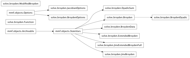
Inheritance diagram for mmf.solve.broyden:
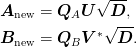
Broyden Root Finders.
This module contains several different root finders that implement Broyden’s method.
Mathematical Background
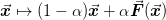
The basic idea is to use a linear approximation to the objective function

where 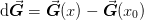 and
and
 .
.
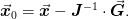
The goal of the Broyden methods is to find the value
 such that
  . This
is done using the Newton step:
. This
is done using the Newton step:
If the Jacobian is exact, then this should give quadratic convergence
as one approaches the root. However, it can be expensive to compute
the Jacobian (at least  function evaluations for a simple
finite difference approximation), so instead, the Broyden method uses
a sequence approximations, starting with the identity and using a
minimal update in the sense of satisfying the secant condition while
minimizing the Frobenius norm of the change. In the following we
shall us bra-ket notation for vectors.
function evaluations for a simple
finite difference approximation), so instead, the Broyden method uses
a sequence approximations, starting with the identity and using a
minimal update in the sense of satisfying the secant condition while
minimizing the Frobenius norm of the change. In the following we
shall us bra-ket notation for vectors.
We shall first discuss the standard Broyden method which imposes a
“minimal” update such that the secant condition  holds.
Standard Broyden Method
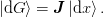
For a given step  where the function changes by
 the update must satisfy the secant condition
We can write any such update in the following form
where  is any vector not orthogonal to .
This ambiguity of the multidimensional secant method causes problems
if not properly resolved, but Broyden showed that good results can be
obtained if the update is chosen to minimize the Frobenius norm of the
Jacobian:
is any vector not orthogonal to .
This ambiguity of the multidimensional secant method causes problems
if not properly resolved, but Broyden showed that good results can be
obtained if the update is chosen to minimize the Frobenius norm of the
Jacobian:
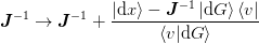
This yields the update
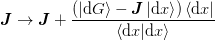
which can be analytically inverted using the Shermann-Morrison formula
to find ![\ket{v} = \left[\mat{J}^{-1}\right]^{T}\ket{\d{x}}](../../../_images/math/c71028ee4666247c20a2e4e44e83f6e6bb1189f7.png) :
:
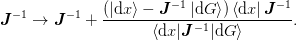
An alternative update (Broyden’s “first” method) is found by minimizing
the norm of the inverse Jacobian, which yields 
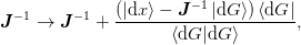
however, we have found that this does not always work as well. It may be used, however, even if the inverse Jacobian develops a singular direction (which can cause trouble for the previous update).
Generalized Broyden Method
This method is a generalization of the one described in
[Bierlaire:2006] and defines the new Jacobian  at the point
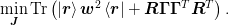
 that minimizes a weighted combination of previous “residuals”
 along with a minimal change condition on a matrix residual
 :
:
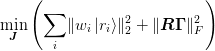
where  are weights and
  will be discussed later and
specifies the weighting of the matrix residual. The residuals may
take the following form:
will be discussed later and
specifies the weighting of the matrix residual. The residuals may
take the following form:
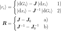
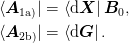
The method 1a) corresponds to the generalization of Broyden’s first or
“Good” method while the combination 2b) corresponds to the
generalization of Broyden’s second or “Bad” method. This second
method with  is the method employed in
[Johnson:1988] with the slight modification that
is the method employed in
[Johnson:1988] with the slight modification that 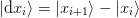 . The two mixed cases 1b) and 2a) are
much more difficult to solve as they are linear in neither
nor
. The two mixed cases 1b) and 2a) are
much more difficult to solve as they are linear in neither
nor  .
.
In what follows, we shall use the notation  for the inverse approximate Jacobian. Boldface capital letters like
this refer to “large”
for the inverse approximate Jacobian. Boldface capital letters like
this refer to “large”  matrices that we typically will not
be able to form. Boldface lowercase letters such as
matrices that we typically will not
be able to form. Boldface lowercase letters such as  denote “small”
  matrices that we can easily
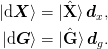
store. We define mixed matrices using bra-ket notation such as
matrices that we can easily
store. We define mixed matrices using bra-ket notation such as
 and
and  for the
  matrices of the vectors
 ![[\ket{\d{\mat{X}}}]_{:i} = \ket{\d{x}_i}](../../../_images/math/ee4c874eaa673ca28fcf9aad58a403dc34f970f0.png) .
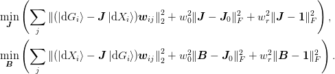
We may now write the minimization condition as:
.
We may now write the minimization condition as:
Using the relationship  we arrive at the following normal equations:
The weights have the following effects:
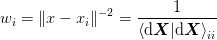
- If not using the subspace decomposition method, then the weights affect the
inversion procedure. In particular, the ratio
 is important for determining the
relative weighting of the old Jacobian and the new steps.
is important for determining the
relative weighting of the old Jacobian and the new steps. - If components of
 and
and  are linearly
dependent – i.e. the secant conditions are not all consistent – them the
weights determine how to mix these.
are linearly
dependent – i.e. the secant conditions are not all consistent – them the
weights determine how to mix these. - If using the subspace decomposition method, then for the linearly independent components, the weights are formally irrelevant, but they can still be used to determine which components should be truncated or ignored (see section Truncation Algorithm). They will also play a role when dynamic restarts are considered (see Dynamic Restarts).
Note
Here we present a little bit of analysis. The first step will be to
define 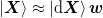 and
and  so that they have full rank and we can write
 ,
,  with
with  and
and  being invertable. (In
the memory limited context, these will be small. They can be computed using
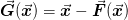
an SVD or rank-revealing QR decomposition.) The two updates can now be
written as:
being invertable. (In
the memory limited context, these will be small. They can be computed using
an SVD or rank-revealing QR decomposition.) The two updates can now be
written as:

The first equality expresses the update as first subtracting off the
projection of the previous approximation on the subspace spanned by
 and then reconstructing this from the new data. In this
sense the update is minimal and can be expressed as minimizing the Frobenius
norm. This follows from equation (1) with
and then reconstructing this from the new data. In this
sense the update is minimal and can be expressed as minimizing the Frobenius
norm. This follows from equation (1) with  .
.
The main feature of this update is that, if the function is linear, then
previous updates will be preserved so that after independent updates,
the approximation will be exact: NO NO NO. Not True!
>>> np.random.seed(0)
>>> import numpy.random
>>> from numpy import mat
>>> from numpy.linalg import svd, qr, inv
>>> ns = numpy.random.randint(1,10,size=10)
>>> N = sum(ns)
>>> X_ = mat(np.random.rand(N,N))
>>> J_ = mat(np.random.rand(N,N))
>>> G_ = J_*X_
>>> B = mat(np.eye(N))
>>> B1 = mat(np.eye(N))
>>> n0 = 0
>>> for n in ns:
...    X = X_[:,n0:n0+n]
...    G = G_[:,n0:n0+n]
...    n0 += n
...    _, g = qr(G)
...    _, x = qr(X)
...    Xhat = svd(X)[0][:,:n]
...    Xperp = svd(X)[0][:,n:]
...    Ghat = svd(G)[0][:,:n]
...    Gperp = svd(G)[0][:,n:]
...    B = B + (X - B*G)*inv(g.T*g)*G.T
...    B1 = B1 - B1*Ghat*Ghat.T + X*inv(g)*Ghat.T
Note
I am trying to form a better intuition for these equations, so
consider the following. First assume that the  is not singular
and that the matrices and are not rank
deficient. (I.e., f there are previous points, then these have rank .
Otherwise, use the weights to reduce the size so that they satisfy this
property appropriately. The weights can now be ignored.) In this case, one
can satisfy the secant conditions exactly if the equations have the following
structure:
is not singular
and that the matrices and are not rank
deficient. (I.e., f there are previous points, then these have rank .
Otherwise, use the weights to reduce the size so that they satisfy this
property appropriately. The weights can now be ignored.) In this case, one
can satisfy the secant conditions exactly if the equations have the following
structure:

for an arbitrary choice of  insofar as
 is not singular. The ambiguity in the choice of
is now captured in the desire to minimize the change from
is not singular. The ambiguity in the choice of
is now captured in the desire to minimize the change from
 and we have:
>>> from numpy.random import rand
>>> from numpy import dot
>>> from numpy.linalg import inv, svd
>>> np.random.seed(0)
>>> dG = rand(5,3)
>>> dX = rand(5,3)
>>> B0 = rand(5,5)
>>> Gamma = dot(svd(dG)[0][:,-2:], rand(2,2))
>>> np.allclose(0, dot(dG.T, Gamma))
True
>>> np.allclose(dot(dG.T, inv(dot(dG, dG.T) + dot(Gamma, Gamma.T))),
...             dot(inv(dot(dG.T, dG)), dG.T))
True
>>> A = dG.T
>>> R = dX - dot(B0, dG)
>>> B1 = B0 + dot(R, dot(inv(dot(A, dG)), A))
[Bierlaire:2006] suggests that a good choice of weights is
something like
which weights the small steps (and hence more likely to be in the
linear regime) more highly than long secant steps. [Johnson:1988]
suggests a similar criterion based on  or a fixed set of
weights depending on iteration number.
or a fixed set of
weights depending on iteration number.
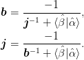
A good choice of and is not so simple,
but we can be lead by the original Broyden method which sets
to be the previous approximate inverse Jacobian.
Another option is to set  or some other
constant independent of iteration. If enough iterates are maintained,
then this might also work (but I am not aware of this method having
been explored).
or some other
constant independent of iteration. If enough iterates are maintained,
then this might also work (but I am not aware of this method having
been explored).
Dynamic Restarts
One interesting idea is to include an additional Jacobian residual
term 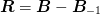 in addition to
  where is constant (typically
 ) and
) and  is the previous
approximation. If we also take
is the previous
approximation. If we also take  ,
then the weight
,
then the weight  will “pull” the inverse Jacobian back towards
. This is useful if one can formulate some slow but
approximately convergent iteration scheme. [Johnson:1988], for
example, advocates restarting the algorithm and resetting the Jacobian
approximation after some progress has been made. Instead, by dynamically
increasing
will “pull” the inverse Jacobian back towards
. This is useful if one can formulate some slow but
approximately convergent iteration scheme. [Johnson:1988], for
example, advocates restarting the algorithm and resetting the Jacobian
approximation after some progress has been made. Instead, by dynamically
increasing  (if the Broyden steps are not improving the residual
for example) once can continuously “restart” the approximation by
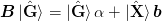
pulling it back toward . This gives the following
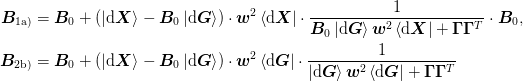
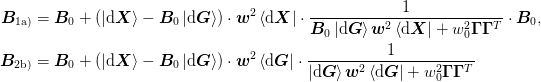
generalized equations (which we express in several forms here):
(if the Broyden steps are not improving the residual
for example) once can continuously “restart” the approximation by
pulling it back toward . This gives the following
generalized equations (which we express in several forms here):
![\mat{J}_{\text{1a)}} &= \Bigl[
\ket{\d\mat{G}}\mat{w}^2\bra{\d\mat{X}}
+ \mat{J}_{-1}\mat{\Gamma}\mat{\Gamma}^{T}
+ \mat{J}_{0}w_0^2
\Bigr]\cdot\Bigl[
\ket{\d\mat{X}}\mat{w}^2\bra{\d\mat{X}}
+ \mat{\Gamma}\mat{\Gamma}^{T}
+ \mat{1}w_0^2
\Bigr]^{-1},\\
&= \mat{J}_{-1} +
\Bigl(
(\ket{\d\mat{G}} - \mat{J}_{-1}\ket{\d\mat{X}})\cdot\mat{w}^2
\bra{\d\mat{X}}
+ (\mat{J}_{0} - \mat{J}_{-1})w_0^2
\Bigr)\cdot\frac{1}{
\ket{\d\mat{X}}\mat{w}^2\bra{\d\mat{X}}
+ \mat{\Gamma}\mat{\Gamma}^{T} + \mat{1}w_0^2},\\
\mat{B}_{\text{1a)}} &= \mat{B}_{-1} +
\Bigl(
(\ket{\d\mat{X}} - \mat{B}_{-1}\ket{\d\mat{G}})\cdot\mat{w}^2
\bra{\d\mat{X}}
+ (\mat{1} - \mat{B}_{-1}\mat{B}_{0}^{-1})w_0^2
\Bigr)\cdot\frac{1}{
\mat{B}_{-1}\ket{\d\mat{G}}\mat{w}^2\bra{\d\mat{X}}
+ \mat{\Gamma}\mat{\Gamma}^{T} + \mat{B}_{-1}\mat{B}_{0}^{-1}w_0^2
}\cdot\mat{B}_{-1}, \\
\mat{B}_{\text{2b)}} &= \Bigl[
\ket{\d\mat{X}}\mat{w}^2\bra{\d\mat{G}}
+ \mat{B}_{-1}\mat{\Gamma}\mat{\Gamma}^{T}
+ \mat{B}_{0}w_0^2
\Bigr]\cdot\Bigl[
\ket{\d\mat{G}}\mat{w}^2\bra{\d\mat{G}}
+ \mat{\Gamma}\mat{\Gamma}^{T}
+ \mat{1}w_0^2
\Bigr]^{-1},\\
&= \mat{B}_{-1} +
\Bigl(
(\ket{\d\mat{X}} - \mat{B}_{-1}\ket{\d\mat{G}})\cdot\mat{w}^2
\bra{\d\mat{G}}
+ (\mat{B}_{0} - \mat{B}_{-1})w_0^2
\Bigr)\cdot\frac{1}{
\ket{\d\mat{G}}\mat{w}^2\bra{\d\mat{G}}
+ \mat{\Gamma}\mat{\Gamma}^{T} + \mat{1}w_0^2
}](../../../_images/math/e79d8850d14e2cb560ed14a313f1649401fe1da7.png)
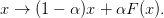
This dynamic restart mechanism can be easily used if one can relate
the objective function  to an approximately
convergent iteration:
to an approximately
convergent iteration:
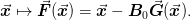
Pulling the approximate inverse Jacobian  will pull the iterations back to this (hopefully)
convergent iteration. Note that the typical linear mixing scheme
will pull the iterations back to this (hopefully)
convergent iteration. Note that the typical linear mixing scheme
 is
simply equivalent to scaling
is
simply equivalent to scaling  which may also be simply implemented.
Note
The diagonals of the matrix  are
specified by the parameter IProblem.j0_scale. The
parameter
are
specified by the parameter IProblem.j0_scale. The
parameter  is treated separately in the solver.
Regularization
Finally, the choice of  is such that the
denominators are positive definite. Several choices are
discussed in [Bierlaire:2006]:
is such that the
denominators are positive definite. Several choices are
discussed in [Bierlaire:2006]:
- “Geometric approach” :
- Here we set
 which is fine unless there are
singular or dependent direction which are common. It is also sufficient with
a dynamic restart where
which is fine unless there are
singular or dependent direction which are common. It is also sufficient with
a dynamic restart where  regularizes the denominator. It is
completely unsuitable, however, for a memory limited approach.
regularizes the denominator. It is
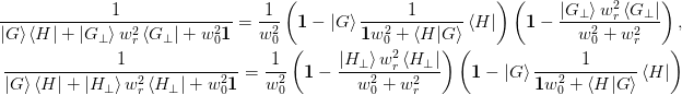
completely unsuitable, however, for a memory limited approach. - “Subspace decomposition” :
The subspace decomposition method makes use of the following formulae:
>>> np.random.seed(0)
>>> w02 = 0.1
>>> wr2 = 0.2
>>> N = 10
>>> m = 5
>>> I = np.eye(N)
>>> i = np.eye(m)
>>> dG = np.mat(np.random.rand(N,m))
>>> H = np.mat(np.random.rand(N,m))
>>> dG_perp = np.linalg.svd(dG)[0][:,m:]
>>> assert(np.allclose(dG.T*dG_perp, 0))
>>> B = np.mat(np.random.rand(N,N))
>>> D = dG*H.T + dG_perp*wr2*dG_perp.T + I*w02
>>> Dinv = ((I - dG*np.linalg.inv(i*w02 + H.T*dG)*H.T)*
...         (I - wr2*dG_perp/(wr2+w02)*dG_perp.T))/w02
>>> np.allclose(D*Dinv,I)
True
>>> H_perp = np.linalg.svd(H)[0][:,m:]
>>> assert(np.allclose(H.T*H_perp, 0))
>>> B = np.mat(np.random.rand(N,N))
>>> D = dG*H.T + H_perp*wr2*H_perp.T + I*w02
>>> Dinv = ((I - wr2*H_perp/(wr2+w02)*H_perp.T)*
...     (I - dG*np.linalg.inv(i*w02 + H.T*dG)*H.T))/w02
>>> np.allclose(D*Dinv,I)
True
For the We start with the subspace decomposition for method 2b). Here we set
 , arriving at the following inversion
formula:
, arriving at the following inversion
formula:The fraction has the following forms for method 1a) and 2b) respectively:
The subspace decomposition method chooses
 to be orthogonal to
either
to be orthogonal to
either  , :math:`
This method sets mat{Gamma} = ket{uvect{X}_{perp}}:math: (case 1a) or mat{Gamma} = ket{uvect{G}_{perp}}:math: (case 1a or 2b). These are the basis vectors orthogonal to ket{dmat{X}}:math: or ket{dmat{G}}:math: respectively. Let the denominator be written as:
(Old notes) A couple of points. First, if w_0 = 0:math:, then the results are independent of the magnitude of mat{Gamma}:math:. To see this, note that one has explicitly (for case 2b) for example):
The second term will be eliminated when acted upon by the numerator factor bra{dmat{G}}:math:. This method poses some formal difficulty for the inversion of the inverse formulation of case 2b) as the denominator contains the mixed term mat{B}_{-1}ket{dmat{G}}mat{w}^2bra{dmat{X}}:math:, however, since one should generally have mat{B}_{-1}ket{dmat{G}} approx ket{dmat{X}}:math:, this should not pose any difficulty in practise. Technically, we implement this by simply performing an SVD of the denominator and dropping the orthogonal subspace.
Note
The standard Broyden method is reproduced with this approach if there is no restart parameter w_0 = 0:math: and only a single previous vector ket{X}:math: is kept.
- “Numerical approach”:
They recommend a numerical approach of performing a Modified Cholesky decomposition mmf.math.linalg.modchol() of mat{A} = ket{dmat{G}}mat{w}^2bra{dmat{X}} = mat{L}mat{L}^{T} - mat{E}:math: where mat{E} = mat{Gamma}mat{Gamma}^T:math: is a diagonal matrix as small as possible making mat{A} + mat{E}:math: safely positive definite and well conditioned.
Unfortunately, this Modified Cholesky based approach does not work for method 1a) where the denominator is both large (Ntimes N:math:) and slightly asymmetric. (Ideally mat{B}_{0}ket{dmat{G}} approx ket{dmat{X}}:math: so the asymmetry should be small.)
Our implementation of this is the same as the “direct inversion” approach discussed below, but with a finite mat{Gamma}:math: such that the smallest singular value is not less than JinvBroyden.min_svd times the largest.
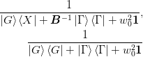
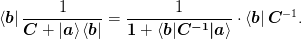
- “Direct inversion”:
If mat{C} = mat{Gamma}mat{Gamma}^{T} + w_{0}^2mat{1}:math: is easily invertible, then the following formula suggested by [Johnson:1988] can be used. (In [Johnson:1988] they set mat{Gamma} = w_{0}mat{1}:math: keeping and so the requirement of minimizing the effect of mat{Gamma}:math: comes in the limit w_0 rightarrow 0:math:. Note that this is not exactly the same as our restart condition because in this case the Jacobian is pulled back to the previous Jacobian, not back to the restart Jacobian.):

>>> from numpy.linalg import inv
>>> np.random.seed(3); N=10; n=3;
>>> X = np.mat(np.random.rand(N, n))
>>> G = np.mat(np.random.rand(N, n))
>>> C = np.mat(np.random.rand(N, N))
>>> I = np.mat(np.eye(N))
>>> i = np.mat(np.eye(n))
>>> np.allclose(inv(C + G*X.T),
...             inv(C) - inv(C)*G*inv(i + X.T*inv(C)*G)*X.T*inv(C))
True
This only requires inverting the small ntimes n:math: matrix mat{1} + braket{mat{X}|mat{mat{G}}}:math:. One further simplification arises when the factor of bra{mat{b}}:math: appears to the left as is the case in both methods without the restart:
(1)
Symmetric Jacobian
If it is known that the Jacobian is symmetric, then this constraint can be built into the minimization with a Lagrange multiplier.
Todo
Finish figuring out how to solve the symmetric problem:
>> A = rand(5,5)
>> B = rand(5,5)
>> B = B+B.T
>> I = eye(5)
>> M = zeros((25,25))
>> for i in xrange(5):
Memory-Limited Extended Broyden Method
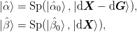
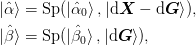
Here we consider a slight generalization of the previous method in a memory limited approach. First, we keep a limited set of n:math: previous points ket{mat{X}}:math: and function evaluations at those points ket{mat{G}}:math:. These define two n-1:math: dimensional subspaces spanned by their differences: ket{uvect{X}} = Spket{deltamat{X}}:math: and ket{uvect{G}} = Spket{deltamat{G}}:math:. This leads to the “stateless” version described first. Second, we keep track of an additional 2m:math: basis vectors for spanning the domain and range of the inverse Jacobian approximation. Thus, we need Ntimes(m+n):math: storage. We express everything in terms of these subspaces, and so work only with (m+n-1)times(m+n-1):math: dimensional matrices as described below. Finally, for simplicity, we assume that the original problem is appropriately scaled so that mat{B}_{0} = mat{1}:math:.
Full “Inefficient” Version
The general update has the form:

where ket{H} in {ket{dmat{X}}, ket{dmat{G}}}:math: for methods 1a) and 2b) respectively.
We start with the subspace decomposition method with mat{Gamma} = ket{G_perp}:math: or mat{Gamma} = ket{H_perp}:math:. The inverse Jacobian has the following general form where ket{R} = ket{dmat{X}} - mat{B}ket{dmat{G}}:math: and ket{H} in {ket{dmat{X}},ket{dmat{G}}}:math: for methods 1a) and 2b) respectively.
>>> np.random.seed(0)
>>> w02 = 0.1
>>> wr2 = 0.2
>>> N = 10
>>> m = 5
>>> I = np.eye(N)
>>> i = np.eye(m)
>>> dG = np.mat(np.random.rand(N,m))
>>> dX = np.mat(np.random.rand(N,m))
>>> H = np.mat(np.random.rand(N,m))
>>> dG_perp = np.linalg.svd(dG)[0][:,m:]
>>> dG_hat = np.linalg.svd(dG)[0][:,:m]
>>> assert(np.allclose(dG.T*dG_perp, 0))
>>> B = np.mat(np.random.rand(N,N))
>>> R = dX - B*dG
>>> B1 = B + (R*H.T + (I-B)*w02)*np.linalg.inv(
...     dG*H.T + dG_perp*wr2*dG_perp.T + I*w02)
>>> f = wr2/(wr2+w02)
>>> B2 = (I + f*(B-I)*(I - dG_hat*dG_hat.T)
...             + (dX - dG)*np.linalg.inv(i*w02 + H.T*dG)*(
...          (1-f)*H.T + f*H.T*dG*np.linalg.inv(dG.T*dG)*dG.T))
>>> np.allclose(B1,B2)
True
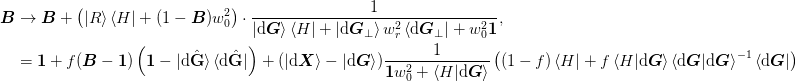
![\begin{aligned}
\mat{B} &\rightarrow
\mat{B} +
\left(\ket{R}\bra{H} + (1-\mat{B})w_0^2\right)\cdot
\frac{1}{\ket{\d\mat{G}}\bra{H} +
\ket{H_\perp}w_{r}^2\bra{H_\perp} + w_0^2\mat{1}} \\
&= \mat{1} + f(\mat{B} - \mat{1})
+ \left[\ket{\d\mat{X}} - \ket{\d\mat{G}}
- f(\mat{B} - \mat{1})
(\ket{\d\mat{G}} + w_0^2\ket{H}\braket{H|H}^{-1})\right]
\frac{1}{\mat{1}w_0^2 + \braket{H|\d\mat{G}}}\bra{H}
\end{aligned}](../../../_images/math/45c21faeda975cf792864dc4afd7faa655bd9aa7.png)
>>> np.random.seed(0)
>>> w02 = 0.1
>>> wr2 = 0.2
>>> N = 10
>>> m = 5
>>> I = np.eye(N)
>>> i = np.eye(m)
>>> dG = np.mat(np.random.rand(N,m))
>>> dX = np.mat(np.random.rand(N,m))
>>> H = np.mat(np.random.rand(N,m))
>>> H_perp = np.linalg.svd(H)[0][:,m:]
>>> H_hat = np.linalg.svd(H)[0][:,:m]
>>> assert(np.allclose(H.T*H_perp, 0))
>>> B = np.mat(np.random.rand(N,N))
>>> R = dX - B*dG
>>> B1 = B + (R*H.T + (I-B)*w02)*np.linalg.inv(
...     dG*H.T + H_perp*wr2*H_perp.T + I*w02)
>>> f = wr2/(wr2+w02)
>>> B2 = (I + f*(B-I)
...         + (dX - dG - f*(B-I)*(dG + w02*H*np.linalg.inv(H.T*H)))
...            *np.linalg.inv(i*w02 + H.T*dG)*H.T)
>>> np.allclose(B1, B2)
True
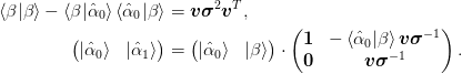
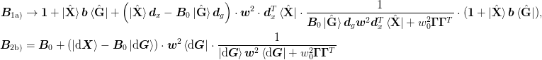
From these expressions we can determine the range and domain of the final inverse Jacobian. Let the previous inverse be expressed as mat{B} = mat{1} + ket{alpha}bra{beta}:math:.
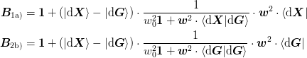
Method 1a)
For method 1a) ket{H} = ket{dmat{X}}mat{w}^2:math:. Choosing mat{Gamma} = ket{uvect{H}_perp}:math: gives the following, which reduces to Broyden’s original “Good” method in the limit of w_0 rightarrow 0:math: and keeping exactly one previous step.
![\mat{B} = \mat{1} + f(\mat{B} - \mat{1})
+ \left[\ket{\d\mat{X}} - \ket{\d\mat{G}}
- f(\mat{B} - \mat{1})
(\ket{\d\mat{G}}
+ w_0^2\ket{\d\mat{X}}
\braket{\d\mat{X}|\d\mat{X}}^{-1}\mat{w}^{-2})\right]
\frac{1}{\mat{1}w_0^2 + \mat{w}^2
\braket{\d\mat{X}|\d\mat{G}}}\mat{w}^2\bra{\d\mat{X}}.](../../../_images/math/32b6605cd39b328fdc00e9c46755b0b45946be9a.png)
The range is Sp(ket{alpha}, ket{dmat{X} - dmat{G}}):math: and the domain is Sp(bra{beta}, bra{dmat{X}}, bra{dmat{G}}):math:. Choosing mat{Gamma} = ket{duvect{G}_perp}:math: gives the following:

The range is Sp(ket{alpha}, ket{dmat{X} - dmat{G}}):math: and the domain is Sp(bra{beta}, bra{dmat{X}}):math:.
Method 2b)
Both expressions are the same for method 2b) since ket{H} = ket{dmat{G}}:math: and the final expression for mat{Gamma} = ket{duvect{G}_perp}:math: is the following, which reduces to Broyden’s original “Bad” method in the limit of w_0 rightarrow 0:math: and keeping exactly one previous step.

The range is Sp(ket{alpha}, ket{dmat{X} - dmat{G}}):math: and the domain is Sp(bra{beta}, bra{dmat{G}}):math:.
Note
These reduce to the following in the limit of f rightarrow 0:math: where one sets w_rrightarrow 0:math:. This limit is a “stateless” version where the Jacobian does not depend on the previous Jacobian (however, in preliminary investigations, this has not performed well.)
>>> np.random.seed(0)
>>> w02 = 0.1
>>> N = 10
>>> m = 5
>>> I = np.eye(N)
>>> dG = np.mat(np.random.rand(N,m))
>>> dX = np.mat(np.random.rand(N,m))
>>> B = np.mat(np.random.rand(N,N))
>>> R = dX - B*dG
>>> w2 = np.mat(np.diag(np.random.rand(m)**2))
>>> B1a = B + (R*w2*dX.T + (I - B)*w02)*np.linalg.inv(
...     B*dG*w2*dX.T + B*w02)*B
>>> B2b = B + (R*w2*dG.T + (I - B)*w02)*np.linalg.inv(
...     dG*w2*dG.T + I*w02)
>>> B1a_ = I + (dX - dG)*np.linalg.inv(
...     np.eye(m)*w02 + w2*dX.T*dG)*w2*dX.T
>>> B2b_ = I + (dX - dG)*np.linalg.inv(
...     np.eye(m)*w02 + w2*dG.T*dG)*w2*dG.T
>>> np.allclose(B1a, B1a_), np.allclose(B2b, B2b_)
True, True
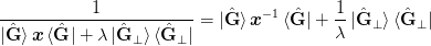
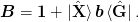
We begin by representing the Jacobian and inverse in a limited subspace as follows:
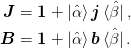
The inversion relation gives
We drop the use of the mat{Gamma}:math: matrix, instead relying on the projectors ket{uvect{alpha}}:math: and ket{uvect{beta}}:math: and minimizing the following
Here we have three weights mat{w}:math: specifies the priority of the secant conditions: This may be a matrix, allowing for more complicated preference schemes involving all n(n-1)/2:math: differences rather than just the n-1:math: basis vectors.
Note
It is assumed that mat{w}:math: is symmetric in this sense that mat{w}^2:math: is used everywhere. The input need not be symmetric and mat{w}^{2} equiv mat{w}mat{w}^T:math: will be used throughout.
Note
In order for this to work well, the Jacobian of the objective function must be well represented by the identity mat{1}:math: plus a correction of low rank. If, for a given problem, the Jacobian has the form mat{J} approx mat{J}_0 + ket{}bra{}:math: then one should rescale the function ket{mat{G}} rightarrow mat{J}_0^{-1} ket{mat{G}}:math: so that the leading term is the identity. It is assumed here that this rescaling has been performed.
This is related to the notion of “linear mixing” as an iterative scheme:
If this is known to converge, then one can probably assume that mat{B} approx alphamat{1} + ket{}bra{}:math: and one should rescale the objective G(x) rightarrow alpha G(x):math:. If this has been done consistently, then pulling the Jacobian back toward the identity with a non-zero w_r:math: will pull the Newton iteration back toward the linear mixing which should restore convergence.
for methods 1a) and 2b) respectively. This gives
From these formula, it is clear that no information will be lost if we have the following:
- 1a)
- 2b)
The purpose of the w_{0}:math: term here is to minimize the change of the approximation from the previous result. This is important for the representation of the Jacobian in the subspace spanned by ket{uvect{alpha}}:math: and ket{uvect{beta}}:math: that lies outside of the space of secant conditions. The parameters w_{r}:math: is new here and “pulls” the solution back toward the identity mat{1}:math: which ideally describes a convergent (but slow) method. This simulates a “restart” when large – resetting the Jacobian to the identity and thus should be used when convergence is poor (or there is a divergence).
The numeric issue here is dealing with poorly behaved matrices. To deal with this, we introduce a parameter singular_tol with the goal that all singular values of the diadic mat{b}:math: of the final inverse Jacobian lie between singular_tol and 1/singular_tol. To do this, all matrix multiplications of the smaller matrices are done using the SVD with singular values outside the range of singular_tol**2 truncated in intermediate calculations and a final truncation within the required range.
Memory-limited Implementation
To limit the amount of memory required, we store the following:
- ket{mat{X}}:math:, ket{mat{G}}:math: :
- N times n:math: matrices: the columns of which are the previous steps and function evaluations. (The oldest steps may be replaced and indices used to keep track of the ordering to minimize the requirement for working with this array.)
- ket{uvect{A}}:math:, ket{uvect{B}}:math: :
- N times m - (n-1):math: matrices representing the extra basis vectors required to span the full space of ket{uvect{alpha}}:math: and ket{uvect{beta}}:math:.
In order to prevent working with the large matrices, we form the following matrices:

Note
This is predicated on the following analysis for extracting the span of a set of vectors. Consider the SVD of a set of vectors:
The desired basis ket{uvect{U}} = Sp(ket{mat{X}}):math: may be expressed in terms of the original vectors as
Hence, we may determine this from the original matrix by considering the eigenvalue decomposition of the small matrix
A rank revealing Cholesky decomposition of braket{mat{X}|mat{X}} = mat{r}^{T}mat{r}:math: may also be similarly used.
A corollary is that, given an orthonormal basis ket{uvect{alpha}_{0}}:math: and a new set of vectors ket{beta}:math:, we may construct the augmented basis by diagonalizing the small matrix
>>> np.random.seed(0)
>>> alpha_0 = np.linalg.qr(np.random.rand(10, 5))[0][:,:5]
>>> beta = np.random.rand(10, 2)
>>> alpha_0_beta = np.dot(alpha_0.T, beta)
>>> s2, v = np.linalg.eigh(np.dot(beta.T, beta)
...                        - np.dot(alpha_0_beta.T, alpha_0_beta))
>>> s = np.sqrt(s2)
>>> alpha_1 = np.dot(beta - np.dot(alpha_0, alpha_0_beta), v/s[None,:])
ket{uvect{alpha}_{0}}:math: and ket{uvect{alpha}_{1}}:math: are orthogonal and normalized:
>>> np.allclose(np.dot(alpha_1.T, alpha_0), 0)
True
>>> np.allclose(np.dot(alpha_1.T, alpha_1), np.eye(2))
True
For large systems, we cannot store the full matrices. If the number of iterations is small, then we can form all of the matrices in terms of dyads (see DyadicSum), however, if the number of iterations becomes too large, then we must truncate the spaces. Let us consider the following information with N:math: being the (large) size of the space, and n:math: be the number of previous steps maintained.
- ket{x}:math:, ket{x_0}:math:, ket{g}:math:, ket{g_0}:math: :
- 1-d arrays of length N of the current and previous steps along with the value of the objective function at these points.
- ket{uvect{X}}:math:, ket{uvect{G}}:math: :
- N times (n-1):math: arrays of orthonormal basis vectors spanning the space of difference vectors ket{x_i} - ket{x_j}:math: and ket{g_i} - ket{g_j}:math: respectively.
- ket{uvect{B}_x}:math:, ket{uvect{B}_g}:math: :
- N times m:math: arrays of orthonormal basis vectors for representing the inverse Jacobian.
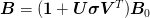
Given these, we can express everything in terms of various n times n:math: matrices in these bases. Thus, the inverse Jacobian is expressed as:
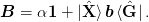
One might like to include an optional preconditioner mat{B} rightarrow mat{B}op{B}_0:math:. For method 1a) the preconditioner factors to the right: to implement this, the simplest approach is to simply precondition the initial function G(x) rightarrow op{B}_{0}G(x):math:. For method 2b) a simple factorization does not work quite as well. [Johnson:1988] also suggests allowing for a factor alpha:math: to reduce the weight of the initial identity approximation:
We now express everything in terms of the basis vectors ket{uvect{X}}:math: and ket{uvect{G}}:math:. Thus, we define the following matrices:
This allows use to express the equations as:
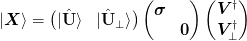
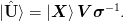
For extremely large systems, we wish to represent the inverse Jacobian as a dyadic sum:
where mat{U}:math: and mat{V}:math: are n times k:math: where n:math: is the size of the problem (large) and k:math: is the number of previous steps we keep (small). The main difficulty with these formula is inverting the large matrix. The “Good” method makes this even more difficult because the denominator is not symmetric while the “Bad” method – apart from possibly suffering some of the numerical instabilities of the “Bad” Broyden method – does not easily allow the form of the dyadic inverse Jacobian to be preserved (if mat{B}_{0}:math: is non-trivial).
Truncation Algorithm
In the memory limited-implementation, one must choose how to discard the previous steps. This choice must be made in two place: the set of previous steps ket{x}:math: and ket{g}:math: to be retained, and the truncation of the current inverse Jacobian approximation mat{B}:math:.
In principle, given n < N:math: previous steps, it is likely that the all of the steps are linearly independent, and so the minimization condition is irrelevant - one simply solves the n:math: secant equations in the subspace spanned by the difference vectors. (The subspace decomposition method has this property - Johnson’s method does not quite have this property when 0 < w_0:math:.)
Once one needs to limit
| [Broyden:1965] | C. G. Broyden, A Class of Methods for Solving Nonlinear Simultaneous Equations, Math. Comput. 19(92), 577-593 (1965) |
| [Johnson:1988] | (1, 2, 3, 4, 5, 6) D. D. Johnson, Modified Broyden’s method for accelerating convergence in self-consistent calculations, Phys. Rev. B 38(18), 12807–12813 (1988) |
| [Bierlaire:2006] | (1, 2, 3) M. Bierlaire, F. Crittin, and M. Themans, A multi-iterate method to solve systems of nonlinear equations, European Journal of Operational Research 183(1), 20 – 41 (2006) |
Parameters
A modification of the Newton step can be used to allow manual control
of some (small) subset of the parameters. As an example (and in our
notations) we consider a set of chemical potentials  and
the respective densities . Allowing the chemical potentials
to change to soon, before the other parameters have relaxed, can throw
off an iteration leading to wild oscillations. Instead, one might
want to wait until a degree of convergence for fixed chemical
potentials has been achieved, and then let the vary.
and
the respective densities . Allowing the chemical potentials
to change to soon, before the other parameters have relaxed, can throw
off an iteration leading to wild oscillations. Instead, one might
want to wait until a degree of convergence for fixed chemical
potentials has been achieved, and then let the vary.
We partition the problem and Jacobian as
The full Broyden step would be to find  and
and  from
from  and
and  using .
Instead, we need to find (and ) from
and the specified “control” parameters .
using .
Instead, we need to find (and ) from
and the specified “control” parameters .
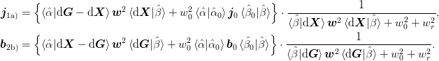
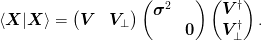
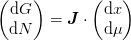
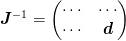
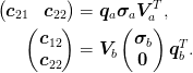
To do this, we partition the inverse Jacobian as
One can solve the problem explicit using the full partitioning, but in
practise, the matrices are large and one can really only form the small
block  corresponding to the small number of control
parameters. The following formula allow one to compute the required
components using only this small matrix, and the inverse Jacobian
(often stored in a compact dyadic representation):
corresponding to the small number of control
parameters. The following formula allow one to compute the required
components using only this small matrix, and the inverse Jacobian
(often stored in a compact dyadic representation):
![\begin{pmatrix}
\d{G}\\
\d{N}
\end{pmatrix} &=
\left(
\mat{1} - \begin{pmatrix}
\mat{0} & \mat{0}\\
\mat{0} & \mat{d}^{-1}
\end{pmatrix}
\left[
\mat{J}^{-1} - \mat{1}\right]
\right)
\cdot
\begin{pmatrix}
\d{G}\\
\d{\mu}
\end{pmatrix}, \\
\begin{pmatrix}
\d{x}\\
\d{\mu}
\end{pmatrix} &=
\mat{J}^{-1}
\cdot
\begin{pmatrix}
\d{G}\\
\d{N}
\end{pmatrix}.](../../../_images/math/6241d6bca15d40f5976d6752b67a939589ddecf8.png)
For calculational purposes we form
Todo
Use scipy.linalg.fblas.dgemm() to allow matrix multiplications etc. to be done in place. In general, minimize memory footprint and make everything work for very large matrices (maybe with an option if it is slower).
Sensitive Parameters
In some situations, certain parameters may be considered “sensitive”. Typically, these are collective parameters. For example, in problems representing functions over a grid, one may have a couple of parameters (such as chemical potentials) where the dependent quantity to be set to zero is an integral of other quantities. Premature optimization of these parameter can cause problems.
A typical case is one where the other “local” parameters must first achieve a certain degree of convergence before the dependent quantity can be accurately estimated. If one attempts to adjust the sensitive parameter before this convergence had been achieved, then the parameters will fluctuate wildly.
What one needs to do is to hold these sensitive parameters fixed for a while, and then adjust them once the local parameters have settled down. In order to ensure that these “noisy” parameters do not mess up the Jacobian, one must call Broyen.update() or Broyden.update_J() with an appropriate argument skip_inds that identifies the noisy parameters. One may use this in conjunction with the previous techniques to provide steps that are consistent with holding these sensitive parameters fixed until the “noise” is sufficiently reduced that updates can be resumed.
Characterizing this “noise” can be tricky: one might for example look for the change in error from a previous iteration. However, if a very small step size has been taken (for example as a result of trying to improve the Jacobian or because of a line-search), then this could result in an incorrect assessment about the degree of convergence.
The simplest criterion is for the case of models where holding the sensitive parameters fixed (and ignoring the error in this component) will lead to a convergent iteration. Here the natural test for”noise” is to check for a weak level of convergence of the other parameters (maybe in conjunction with the change in the parameter error change from iteration to iteration). This is equivalent to an efficient method of solving the following recursive problem: Define an outer problem with only the sensitive parameters. The objective function solves the inner problem with these parameters fixed, then the outer problem solves for the sensitive parameters.
Linear Algebra
Here we summarize some of the linear algebra required here.
Subspace Reduction
One of the problems we shall encounter is that we have a matrix expressed in a basis as
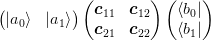
and we need to reduce the rank of the subspaces ket{a_1}:math: and bra{b_1}:math: while holding subspaces ket{a_0}:math: and bra{b_0}:math: fixed. I am not yet sure what the optimal solution to this problem is, but a very good solution can be obtained by performing two SVD’s:
The truncation scheme is then to use the two transformations obtained to determine the rearrangement. This typically approaches the optimal truncation to within a couple of percent (though a tuned matrix could probably break this).
To demonstrate this, we project out one state from a 4 by 4 matrix. We compute the optimal projection using a non-linear solver:
>>> np.random.seed(0)
>>> def my_projection(A):
...     A = np.asmatrix(A)
...     P = np.asmatrix(np.diag([1.0, 1.0, 1.0, 0.0]))
...     qa, _, _ = np.linalg.svd(A[2:,:])
...     _, _, qbt = np.linalg.svd(A[:,2:])
...     Qa = Qbt = np.eye(4)
...     Qa[2:,2:] = qa
...     Qbt[2:, 2:] = qbt
...     return Qa*P*Qa.T*A*Qbt.T*P*Qbt
>>> solver = sp.optimize.fmin_powell
>>> def optimal_projection(A):
...     P = np.asmatrix(np.diag([1.0, 1.0, 1.0, 0.0]))
...     def trans(A, x):
...         t1, t2 = x
...         qa = np.mat([[np.cos(t1), -np.sin(t1)],
...                      [np.sin(t1), np.cos(t1)]])
...         qbt = np.mat([[np.cos(t2), -np.sin(t2)],
...                       [np.sin(t2), np.cos(t2)]])
...         Qa = Qbt = np.eye(4)
...         Qa[2:,2:] = qa
...         Qbt[2:,2:] = qbt
...         return Qa.T*P*Qa*A*Qbt.T*P*Qbt
...     def f(x):
...         return np.linalg.norm(trans(A,x) - A, 2)
...     x = solver(f, [0, 0], disp=False)
...     return trans(A, x)
>>> def rel_err(A):
...     e1 = np.linalg.norm(my_projection(A) - A, 2)
...     e0 = np.linalg.norm(optimal_projection(A) - A, 2)
...     return(abs(e0-e1)/abs(e0))
>>> errs = []
>>> for n in xrange(10):
...     #print("%i of 10" % n)
...     errs.append(rel_err(np.random.rand(4,4) - np.random.rand(4,4)))
>>> np.mean(errs), np.std(errs), np.max(errs) < 0.1
(0.01..., 0.02..., True)
To do this we note that we can perform a block diagonalization
of the matrix using the SVD of the lower-right block mat{c}_{22} = mat{u}mat{sigma}mat{v}^{T}:math: and truncating the basis based on this. This follows from the following decomposition:

Notes
Here we summarize some problems, convergence characteristics etc.
In one case we got stuck in a loop adding a point that was already included. What happened is that we were using JinvBroyden.x_method =’min’ which was choosing a particular point. A step was made from this point producing a new point which was added, but the new point did not have a lower `norm{G(x)}$ so the same point was used over and over again with no significant update to the Jacobian.
A similar problem can occur with JinvBroyden.replace_method =’largest’. The resolution consists of one of the following:
- Using to JinvBroyden.x_method = ‘recent’ and JinvBroyden.replace_method =’oldest’ to ensure that that all the points are cycled through and that the newest point is used. These are now the defaults.
- Using a line-search to ensure that a downhill step is chosen to ensure that the newest points have the smallest error.
To Do
Todo
Check why things work better with limited memory options. I.e. keeping a large JinvBroyden.n_prev can make things worse.
- class mmf.solve.broyden.DyadicSum(*varargin, **kwargs)[source]
Bases: mmf.objects.StateVars
Represents a matrix as a sum of
dyads of length :DyadicSum(at=[], b=[], sigma=[], n_max=inf, inplace=False, use_svd=True, dynamic_range=2.22044604925e-16)
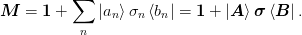
The two sets of bases are stored in
matrices
 and
and  and the matrix
 .
.If use_svd is True, then the singular value decomposition of
is used to keep
diagonal with positive entries and only these diagonals are stored.Todo
Perform an analysis of the inverse jacobian, changing bases if needed to make the dyads linearly independent.
Note
We assume everything is real here: no complex conjugation is performed with transposition.
Examples
>>> J = DyadicSum()
>>> x = np.mat([[1.0],
...             [2.0]])
>>> J*x - x
matrix([[ 0.],
        [ 0.]])
>>> b = np.mat([[1.0, 0.0]])
>>> a = np.mat([[0.0],
...             [2.0]])
>>> J.add_dyad(a, b)
>>> J*x
matrix([[ 1.],
        [ 4.]])
>>> x.T*J
matrix([[ 5.,  2.]])
>>> import mmf.archive
>>> A = mmf.archive.Archive()
>>> A.insert(J=J)
'J'
>>> s = str(A)
>>> d = {}
>>> exec(s, d)
>>> np.allclose(J.asarray(), d['J'].asarray())
True
Here is an example of limiting the size of the dyadic.
>>> np.random.seed(3)
>>> s1 = np.eye(10)
>>> s2 = DyadicSum(n_max=10)
>>> for n in xrange(100):
...    a = np.random.random(10)
...    b = np.random.random(10)
...    _add_dyad(s1, a, b)
...    s2.add_dyad(a, b)
This should still be exact because the space is only ten dimensional.
>>> np.allclose(s1, s2.asarray())
True
The dynamic_range parameter is a more mathematical way of keeping the basis fixed. It ensures that the most significant singular values will be kept.
>>> s1 = DyadicSum(dynamic_range=0.01)
>>> s2 = DyadicSum()
>>> for n in xrange(100):
...    a = np.random.random(20)
...    b = np.random.random(20)
...    s1.add_dyad(a, b)
...    s2.add_dyad(a, b)
>>> d1 = np.linalg.svd(s1.asarray(), compute_uv=False)
>>> d2 = np.linalg.svd(s2.asarray(), compute_uv=False)
>>> (abs(d1 - d2)/max(d2)).max() < 0.02
True
Attributes
State Variables: - at
(N, n) array . We use the ket form here because
that is most often used and more efficient (presently,
numpy.dot() makes copies if the arrays are not both
C_CONTIGUOUS.- b
(n, N) array  .
.- sigma
(n, n) array or (n, ) array  if use_svd.
- n_max
Maximum number of Dyads to store. If this is finite, then the
matrices are pre-allocated, and when  new dyads are
added, they replace the least significant dyads, requiring no
more allocations, otherwise the dyads are added as required.
new dyads are
added, they replace the least significant dyads, requiring no
more allocations, otherwise the dyads are added as required.- inplace
If n_max is finite, then this signifies that the matrices at and b should be allocated only once and all operations should be done inplace on these. In particular, when new dyads are added, the least significant components of the ole matrix are dropped first then the dyads are added.
If this is False, then the new dyads are added first and then the least-significant components are dropped. This latter form requires more storage, but may be more accurate.
Note
Presently, the inplace operations cannot be performed because scipy does not expose the correct BLAS routines, so the only purpose of this flag is to somewhat limit memory usage, but this is probably quite ineffective at the moment.
- use_svd
If True, then orthogonalize() will be run whenever a new dyad is added. (Generally a good idea, but can be slow if there are a lot of dyads). - dynamic_range
Each call to orthogonalize() will only keep the singular values within this fraction of the highest. Methods
add_dyad(at, b[, sigma]) Add |a>d<b| to J. all_items() Return a list [(name, obj)] of (name, object) pairs containing all items available. apply_transform(f[, fr]) Apply the linear transform f to the vectors forming the dyads. archive(name) Return a string representation that can be executed to restore the object. archive_1([env]) Return (rep, args, imports). asarray() Return the matrix. diag([k]) Return the diagonal of the matrix. initialize(**kwargs) Calls __init__() passing all assigned attributes. items([archive]) Return a list [(name, obj)] of (name, object) pairs where the orthogonalize([at, b, sigma]) Perform a QR decomposition of the dyadic components to reset() Reset the matrix. resume() Resume calls to __init__() from __setattr__(), suspend() Suspend calls to __init__() from - add_dyad(at, b, sigma=None)[source]
Add |a>d<b| to J.
Parameters : at, b : array
These should be either 1-d arrays (for a single dyad) or 2-d arrays ((N, m) for at and (m, N) for b) arrays representing the bra’s <a| and <b|.
sigma : array
Matrix linking at and b. Must be provided if len(at.T) and len(b) are different.
Examples
Here is a regression test for a bug: adding a set of dyads that would push the total number beyond n_max.
>>> np.random.seed(0)
>>> at = np.random.random((10, 3))
>>> b = np.random.random((3, 10))
>>> s = DyadicSum(n_max=2)
>>> s.add_dyad(at=at, b=b)
- apply_transform(f, fr=None)[source]
Apply the linear transform f to the vectors forming the dyads. If fr is None, this is applied to the right (bra’s), otherwise f is applied to both sides. This is equivalent to the transformation J ->I + F*(J - I)*Fr.T.
Note
This should be modified to be done in place if possible.
- asarray()[source]
Return the matrix.
Examples
>>> M = DyadicSum()
>>> M.asarray()
array(1.0)
>>> M.add_dyad([1, 0], [1, 0])
>>> M.add_dyad([0, 2], [1, 0])
>>> M.add_dyad([3, 0], [0, 1])
>>> M.add_dyad([0, 4], [0, 1])
>>> M.asarray()
array([[ 2.,  3.],
       [ 2.,  5.]])
- diag(k=0)[source]
Return the diagonal of the matrix.
Examples
>>> M = DyadicSum()
>>> M.diag()
array(1.0)
>>> M.add_dyad([1, 0], [1, 0])
>>> M.add_dyad([0, 2], [1, 0])
>>> M.add_dyad([3, 0], [0, 1])
>>> M.add_dyad([0, 4], [0, 1])
>>> M.diag()
array([ 2.,  5.])
- orthogonalize(at=None, b=None, sigma=None)[source]
Perform a QR decomposition of the dyadic components to make them orthogonal.
Notes

In order to compute the QR factorization of
without working with the large matrices, we could do a Cholesky
decomposition on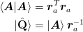
Note
These should be nicely accelerated using the BLAS routines for performing the operations in place. In principle, numpy.dot() should do this, but at present there are issues with contiguity that force copies to be made. Also, SciPy does not yet expose all BLAS operations, in particular _SYRK is missing.
We perform a QR decomposition of these

and then an SVD of the product of the R factors
 to obtain the new basis:
- reset()[source]
Reset the matrix.
Examples
>>> M = DyadicSum()
>>> M.asarray()
array(1.0)
>>> M.add_dyad([1, 0], [1, 0])
>>> M.add_dyad([0, 2], [1, 0])
>>> M.add_dyad([3, 0], [0, 1])
>>> M.add_dyad([0, 4], [0, 1])
>>> M.asarray()
array([[ 2.,  3.],
       [ 2.,  5.]])
>>> M.reset()
>>> M.asarray()
array(1.0)


- class mmf.solve.broyden.JinvBroyden(*varargin, **kwargs)[source]
Bases: mmf.objects.StateVars
Class to represent an inverse Jacobian for the Generalized Broyden method.
JinvBroyden(curr=None,
            xs=None,
            gs=None,
            n_prev=10,
            method=J,
            x_method=recent,
            replace_method=oldest,
            inv_method=svd,
            min_svd=1e-08,
            w0=1,
            w_min=1.49011611938e-08,
            dyadic=False,
            j_inv=1,
            robust=False,
            max_j_inv=100.0,
            min_j_inv=0.0001,
            minimize_inverse=False,
            incompatibility_measure=dg,
            check_roundoff=True,
            roundoff_cut=0.001,
            _j_inv_transform=,
            _dx_norm2_min=4.93038065763e-32,
            _age=None,
            _x0=None,
            _g0=None)
This is intended to solve root-finding problems of the form

This is designed for large scale problems where it is typically prohibitive to store the entire Jacobian, so a limited memory approximation is typically made by using dyadic and n_prev. As a result, we assume that the problem is preconditions so that the Jacobian is well approximated by the identity.

In other words, we implicitly expect that the problem is preconditioned in such a way that
where the iteration
 is
“almost” convergent. This assumption plays out in much of the
internal analysis about when behaviour is singular.
is
“almost” convergent. This assumption plays out in much of the
internal analysis about when behaviour is singular.The core of this is one of the following two updates to the inverse Jacobian:
where the weights
 are computed using _get_weight()
and the inversion of the denominator is computed using
_inversion(). The displacements are computed from the
current step
are computed using _get_weight()
and the inversion of the denominator is computed using
_inversion(). The displacements are computed from the
current step  and
and  and the previous steps
 and
and  , of which we store the
previous n_prev steps.
, of which we store the
previous n_prev steps.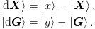
Examples
We start with a linear function. The Jacobian should fully represent this.
>>> np.random.seed(0)
>>> A = np.random.random((3, 3))
>>> Ainv = np.linalg.inv(A)
>>> b = np.random.random(3)
>>> x0 = np.random.rand(3)
>>> def g(x):
...     return np.dot(A, x) + b
For both method “good” (‘J’) and “bad” (‘B’) the inv_method ‘svd’ reproduces the Jacobian once the full space is sampled:
>>> B = JinvBroyden(dyadic=True, inv_method='svd')
>>> for B.method in ['J', 'B']:
...     B.reset_all()
...     x_ = 1*x0
...     for n in xrange(4):
...         g_ = g(x_)
...         incompatibility = B.set_point(x=x_, g=g_)
...         x_ = B.get_x()
...     np.allclose(B.j_inv.asarray(), Ainv)
True
True
The inv_method ‘w0’ does not exactly reproduce this as it “remembers” the initial Jacbian
 , but the results are
almost correct if w0 is small enough:
, but the results are
almost correct if w0 is small enough:>>> B.inv_method = 'w0' >>> B.x_method = 'recent' >>> B.w0 = 0.0001 >>> for B.method in ['J', 'B']: ... B.reset_all() ... x_ = 1*x0 ... for n in xrange(4): ... g_ = g(x_) ... incompatibility = B.set_point(x=x_, g=g_) ... x_ = B.get_x() ... # abs(B.j_inv.asarray() - Ainv).max() ... print(np.allclose(B.j_inv.asarray(), Ainv), ... np.allclose(B.j_inv.asarray(), Ainv, atol=0.001), ... np.allclose(B.j_inv.asarray(), Ainv, atol=0.003)) (False, True, True) (False, False, True)
This also demonstrates that the “good” method 1a) converges better to the Jacobian.
Here we start with a non-trivial Jacobian but no vectors xs and then update. This happens, for example, with change_basis(). We only keep xs and gs for exact x = g(x) and this is violated by linear changes in the basis, so we discard the points but keep the Jacobian.
>>> np.random.seed(0)
>>> B = JinvBroyden(dyadic=False, inv_method='svd', method='B')
>>> B0 = np.random.random((4, 4))
>>> B.j_inv = 1*B0
>>> x = np.random.random(4)
>>> g = np.random.random(4)
>>> B.set_point(x=x, g=g)
0.0
This does not yet modify the Jacobian because we have only one point
>>> abs(B0 - B.j_inv).max()
0.0
Now we update the Jacobian
>>> dx = np.random.random(4)
>>> dg = np.random.random(4)
>>> B.set_point(x=x+dx, g=g+dg)
0.79...
The new Jacobian now fits the slope properly,
>>> np.allclose(B.j_inv*dg[:, None], dx[:, None])
True
But has not been modified in orthogonal directions (only true for method ‘B’).
>>> dg_perp = np.linalg.qr(np.vstack([dg, np.random.random(4)]).T)[0][:, 1]
>>> np.allclose(np.dot(dg_perp, dg), 0)
True
>>> np.allclose(np.dot(B0, dg_perp[:, None]), B.j_inv*dg_perp[:, None])
True
If you want to reproduce the original Broyden algorithms, then one should set: n_prev to 2, x_method to ‘recent’, inv_method to ‘svd’, and replace_method to ‘oldest’.
Attributes
- class mmf.solve.broyden.ExtendedBroyden(*varargin, **kwargs)[source]
Bases: mmf.objects.StateVars
This is a class implementing the memory limited extended Broyden update.
ExtendedBroyden(method=1)
Attributes
- class mmf.solve.broyden._JinvExtendedBroyden(*varargin, **kwargs)[source]
Bases: mmf.objects.StateVars
Class to represent an inverse Jacobian for the Extended Broyden method. Presently, this class does not do any of the special processing to minimize the memory footprint described in the module description.
_JinvExtendedBroyden(X=Required,
                     G=Required,
                     _b=None,
                     method=1,
                     n_prev_steps=inf,
                     _check=True)
We represent the inverse Jacobian as:
Notes
Since python is implemented in C, the arrays are typically stored as C_CONTIGUOUS and numpy.dot() is efficient if both arguments are C_CONTIGUOUS, otherwise copies are made. Thus, where one needs to compute
 , one should
store the transpose of the first matrix .
, one should
store the transpose of the first matrix .Attributes
State Variables: - X
 array of previous steps
  .
.- G
array of objectives  .
.- _b
Dyadic portion of the inverse Jacobian in the implied basis. - method
1 for Broyden’s good method and 2 for the “bad” method. - n_prev_steps
Number of previous steps to keep and use.- _check
If True, perform some potentially expensive sanity checks. Delegates: - _JinvExtendedBroyden._jinv = DyadicSum()
<no description> References: - _JinvExtendedBroyden.at -> _JinvExtendedBroyden._jinv.at
(N, n) array . We use the ket form here because
that is most often used and more efficient (presently,
numpy.dot() makes copies if the arrays are not both
C_CONTIGUOUS.- _JinvExtendedBroyden.b -> _JinvExtendedBroyden._jinv.b
(n, N) array .- _JinvExtendedBroyden.sigma -> _JinvExtendedBroyden._jinv.sigma
(n, n) array or (n, ) array
if use_svd.- _JinvExtendedBroyden.n_max -> _JinvExtendedBroyden._jinv.n_max
Maximum number of Dyads to store. If this is finite, then the
matrices are pre-allocated, and when new dyads are
added, they replace the least significant dyads, requiring no
more allocations, otherwise the dyads are added as required.- _JinvExtendedBroyden.inplace -> _JinvExtendedBroyden._jinv.inplace
If n_max is finite, then this signifies that the matrices at and b should be allocated only once and all operations should be done inplace on these. In particular, when new dyads are added, the least significant components of the ole matrix are dropped first then the dyads are added.
If this is False, then the new dyads are added first and then the least-significant components are dropped. This latter form requires more storage, but may be more accurate.
Note
Presently, the inplace operations cannot be performed because scipy does not expose the correct BLAS routines, so the only purpose of this flag is to somewhat limit memory usage, but this is probably quite ineffective at the moment.
- _JinvExtendedBroyden.use_svd -> _JinvExtendedBroyden._jinv.use_svd
If True, then orthogonalize() will be run whenever a new dyad is added. (Generally a good idea, but can be slow if there are a lot of dyads). - _JinvExtendedBroyden.dynamic_range -> _JinvExtendedBroyden._jinv.dynamic_range
Each call to orthogonalize() will only keep the singular values within this fraction of the highest. Methods
all_items() Return a list [(name, obj)] of (name, object) pairs containing all items available. archive(name) Return a string representation that can be executed to restore the object. archive_1([env]) Return (rep, args, imports). asarray() Return the Jacobian matrix. get_w(dXdX, dGdG) Return weights w, w0, wr. initialize(**kwargs) Calls __init__() passing all assigned attributes. items([archive]) Return a list [(name, obj)] of (name, object) pairs where the resume() Resume calls to __init__() from __setattr__(), suspend() Suspend calls to __init__() from update([x0, g0]) Update the inverse Jacobian so that it is valid at the - asarray()[source]
Return the Jacobian matrix.
Examples
>>> M = _JinvExtendedBroyden()
>>> M.asarray()
array(1.0)
- update(x0=None, g0=None)[source]
Update the inverse Jacobian so that it is valid at the point (x, g).
Return a measure of the incompatibility of the new data with the current approximation.
Notes
Our goal here is to minimize the amount of processing of large matrices. As such, we try to work with projections as much as possible. We start with the following large matrices:
,  , , ,
, , ,  ,
,
 .
.We use the following:
Examples
Here we perform some tests with a linear function
>>> np.random.seed(0)
>>> N = 4
>>> J = np.random.rand(N, N)
>>> x0 = np.random.rand(N)
>>> def g(x):
...     return np.dot(J, x - x0)
>>> B = _JinvExtendedBroyden(X=np.zeros((N,1)),
...                         G=g(0*x0)[:,None])
>>> x = np.random.rand(N)
>>> B.update(x, g(x))
>>> np.allclose(B*(g(x) - g(x0)), x - x0)
True
>>> for n in xrange(N):
...     x = np.random.rand(N)
...     B.update(x, g(x))
- class mmf.solve.broyden.JinvExtendedBroydenFull(*varargin, **kwargs)[source]
Bases: mmf.objects.StateVars
Class to represent an inverse Jacobian for the Extended Broyden method using full matrices (for small problems only).
JinvExtendedBroydenFull(curr=None,
                        xs=[],
                        gs=[],
                        j_inv=None,
                        j_inv0=1.0,
                        method=J,
                        n_prev=1000,
                        max_j_inv=100.0,
                        min_j_inv=0.0001,
                        _eps=2.22044604925e-16,
                        _x0=None,
                        _g0=None)
Attributes