`mmf.physics.potentials.separable`¶

`VPoschlTeller`(varargin, *kwargs)	Poschl-Teller potential used by GFMC groups.
`Separable`(varargin, *kwargs)	Base class for separable potentials, including methods to compute their scattering properties: $a^{-1}$ and $r_{eff}$ are computed by `potentials.ainv()` and `potentials.reff()`.
`SharpCutoff`(varargin, *kwargs)	Separable potential with a sharp momentum cutoff.
`SmoothCutoff`(varargin, *kwargs)	Separable potential with a smooth momentum cutoff.
`Yamaguchi`(varargin, *kwargs)	Separable Yamaguchi potential.
`EffectiveRange`(varargin, *kwargs)	Separable Effective Range Interaction, completely determined by the scattering length and effective range.

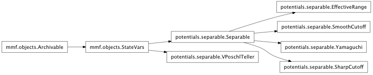
Inheritance diagram for mmf.physics.potentials.separable:

Inheritance diagram of mmf.physics.potentials.separable

Separable Potentials.

This module contains various three-dimensional separable potentials of the form

$\op{V} = g V_k V_q$

The relevant one-body Schrodinger equation becomes in momentum space (for bound states):

System Message: WARNING/2 (\left(\frac{k}{2m} - E\right)\psi_k = -gV_k \int\dbar^{3}{\vect{q}}\;V_q\psi_q.)

latex exited with error: [stderr] [stdout] This is pdfTeX, Version 3.1415926-2.4-1.40.13 (TeX Live 2012) restricted \write18 enabled. entering extended mode (./math.tex LaTeX2e <2011/06/27> Babel <v3.8m> and hyphenation patterns for english, dumylang, nohyphenation, ge rman-x-2012-05-30, ngerman-x-2012-05-30, afrikaans, ancientgreek, ibycus, arabi c, armenian, basque, bulgarian, catalan, pinyin, coptic, croatian, czech, danis h, dutch, ukenglish, usenglishmax, esperanto, estonian, ethiopic, farsi, finnis h, french, friulan, galician, german, ngerman, swissgerman, monogreek, greek, h ungarian, icelandic, assamese, bengali, gujarati, hindi, kannada, malayalam, ma rathi, oriya, panjabi, tamil, telugu, indonesian, interlingua, irish, italian, kurmanji, latin, latvian, lithuanian, mongolian, mongolianlmc, bokmal, nynorsk, polish, portuguese, romanian, romansh, russian, sanskrit, serbian, serbianc, s lovak, slovenian, spanish, swedish, turkish, turkmen, ukrainian, uppersorbian, welsh, loaded. (/usr/local/texlive/2012/texmf-dist/tex/latex/base/article.cls Document Class: article 2007/10/19 v1.4h Standard LaTeX document class (/usr/local/texlive/2012/texmf-dist/tex/latex/base/size12.clo)) (/usr/local/texlive/2012/texmf-dist/tex/latex/base/inputenc.sty (/usr/local/texlive/2012/texmf-dist/tex/latex/ucs/utf8x.def)) (/usr/local/texlive/2012/texmf-dist/tex/latex/ucs/ucs.sty (/usr/local/texlive/2012/texmf-dist/tex/latex/ucs/data/uni-global.def)) (/usr/local/texlive/2012/texmf-dist/tex/latex/amsmath/amsmath.sty For additional information on amsmath, use the `?’ option. (/usr/local/texlive/2012/texmf-dist/tex/latex/amsmath/amstext.sty (/usr/local/texlive/2012/texmf-dist/tex/latex/amsmath/amsgen.sty)) (/usr/local/texlive/2012/texmf-dist/tex/latex/amsmath/amsbsy.sty) (/usr/local/texlive/2012/texmf-dist/tex/latex/amsmath/amsopn.sty)) (/usr/local/texlive/2012/texmf-dist/tex/latex/amscls/amsthm.sty) (/usr/local/texlive/2012/texmf-dist/tex/latex/amsfonts/amssymb.sty (/usr/local/texlive/2012/texmf-dist/tex/latex/amsfonts/amsfonts.sty)) (/usr/local/texlive/2012/texmf-dist/tex/latex/tools/bm.sty) (/Users/mforbes/Library/texmf/tex/latex/mmf/mmfmath.sty (/usr/local/texlive/2012/texmf-dist/tex/latex/mh/mathtools.sty (/usr/local/texlive/2012/texmf-dist/tex/latex/graphics/keyval.sty) (/usr/local/texlive/2012/texmf-dist/tex/latex/tools/calc.sty) (/usr/local/texlive/2012/texmf-dist/tex/latex/mh/mhsetup.sty)) (/usr/local/texlive/2012/texmf-dist/tex/latex/base/ifthen.sty) (/usr/local/texlive/2012/texmf-dist/tex/latex/doublestroke/dsfont.sty) (/usr/local/texlive/2012/texmf-dist/tex/generic/mathdots/mathdots.sty)) (/usr/local/texlive/2012/texmf-dist/tex/latex/preview/preview.sty) No file math.aux. (/usr/local/texlive/2012/texmf-dist/tex/latex/ucs/ucsencs.def) (/usr/local/texlive/2012/texmf-dist/tex/latex/graphics/graphicx.sty (/usr/local/texlive/2012/texmf-dist/tex/latex/graphics/graphics.sty (/usr/local/texlive/2012/texmf-dist/tex/latex/graphics/trig.sty) (/usr/local/texlive/2012/texmf-dist/tex/latex/latexconfig/graphics.cfg) (/usr/local/texlive/2012/texmf-dist/tex/latex/graphics/dvips.def))) Preview: Fontsize 12pt (/usr/local/texlive/2012/texmf-dist/tex/latex/amsfonts/umsa.fd) (/usr/local/texlive/2012/texmf-dist/tex/latex/amsfonts/umsb.fd) ! LaTeX Error: Command \dj unavailable in encoding OT1. See the LaTeX manual or LaTeX Companion for explanation. Type H <return> for immediate help. ... l.19 \end{gather} ! LaTeX Error: Command \dj unavailable in encoding OT1. See the LaTeX manual or LaTeX Companion for explanation. Type H <return> for immediate help. ... l.19 \end{gather} [1] (./math.aux) ) (see the transcript file for additional information) Output written on math.dvi (1 page, 668 bytes). Transcript written on math.log.

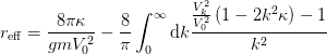
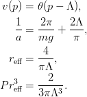
The effective range expansion can be expressed succinctly for separable potentials:

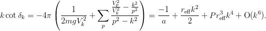
$k\cot\delta_k = -4\pi\left(\frac{1}{2 m g V_k^2} + \sum_{p}\frac{\frac{V_p^2}{V_k^2} - \frac{k^2}{p^2}} {p^2 - k^2}\right) = \frac{-1}{a} + \frac{r_{\text{eff}}k^2}{2} + P r_{\text{eff}}^{3}k^{4} + \order(k^6).$

The first two coefficients are computed by the methods Separable.ainv() and Separable.reff().

Note

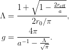
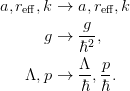
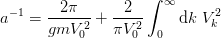
Everything here is expressed in units where $\hbar=1$ . To restore these constants make the following substitutions. Also, these units are for the one-body problem: i.e. $m$ is the mass of a single species. If you wish to use these for the two-body problem, be sure to use the reduced mass in place of $m$ .

$a, r_{\text{eff}}, k & \rightarrow a, r_{\text{eff}}, k\\ g &\rightarrow \frac{g}{\hbar^2},\\ \Lambda, p & \rightarrow \frac{\Lambda}{\hbar}, \frac{p}{\hbar}.$

The dimensions are thus:

[ $\hbar$ ] :

$ET = ML^2/T = 1$ which implies $T \equiv ML^2$ .

[ $v$ ] :

$1$

[ $g$ ] :

$EV = ML^5/T^2 = 1/T = L/M$ .

[ $a$ ] = [ $r_e$ ] :

$1/L$

class mmf.physics.potentials.separable.VPoschlTeller(*varargin, **kwargs)[source]¶

Bases: mmf.objects.StateVars

Poschl-Teller potential used by GFMC groups.

VPoschlTeller(V0=-1.0,
              r0=Required)

Attributes

State Variables:
`V0`¶	Strength of the potential.
`r0`¶	Range of potential. (This is only the effective range if V0 = -1)

Methods

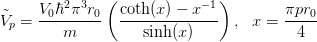
`V`(r[, m])
`Vp`(p[, m])	Fourier transform of potential.
`Vpq`(p, q[, m])	Integrated potential over angles that appears in the BCS
`all_items`()	Return a list [(name, obj)] of (name, object) pairs containing all items available.
`archive`(name)	Return a string representation that can be executed to restore the object.
`archive_1`([env])	Return (rep, args, imports).
`initialize`(**kwargs)	Calls `__init__()` passing all assigned attributes.
`items`([archive])	Return a list [(name, obj)] of (name, object) pairs where the
`resume`()	Resume calls to `__init__()` from `__setattr__()`,
`suspend`()	Suspend calls to `__init__()` from

This is the initialization routine. It is called after the attributes specified in _state_vars have been assigned.

The user version should perform any after-assignment initializations that need to be performed.

Note

Since all of the initial arguments are listed in kwargs, this can be used as a list of attributes that have “changed” allowing the initialization to be streamlined. The default __setattr__() method will call __init__() with the changed attribute to allow for recalculation.

This recomputing only works for attributes that are assigned, i.e. iff __setattr__() is called. If an attribute is mutated, then __getattr__() is called and there is no (efficient) way to determine if it was mutated.

Computed values with True Computed.save will be passed in through kwargs when objects are restored from an archive. These parameters in general need not be recomputed, but this opens the possibility for an inconsistent state upon construction if a user inadvertently provides these parameters. Note that the parameters still cannot be set directly.

See __init__() Semantics for details.

Methods

`V`(r[, m])
`Vp`(p[, m])	Fourier transform of potential.
`Vpq`(p, q[, m])	Integrated potential over angles that appears in the BCS
`all_items`()	Return a list [(name, obj)] of (name, object) pairs containing all items available.
`archive`(name)	Return a string representation that can be executed to restore the object.
`archive_1`([env])	Return (rep, args, imports).
`initialize`(**kwargs)	Calls `__init__()` passing all assigned attributes.
`items`([archive])	Return a list [(name, obj)] of (name, object) pairs where the
`resume`()	Resume calls to `__init__()` from `__setattr__()`,
`suspend`()	Suspend calls to `__init__()` from

__init__(*varargin, **kwargs)¶

This is the initialization routine. It is called after the attributes specified in _state_vars have been assigned.

The user version should perform any after-assignment initializations that need to be performed.

Note

Since all of the initial arguments are listed in kwargs, this can be used as a list of attributes that have “changed” allowing the initialization to be streamlined. The default __setattr__() method will call __init__() with the changed attribute to allow for recalculation.

This recomputing only works for attributes that are assigned, i.e. iff __setattr__() is called. If an attribute is mutated, then __getattr__() is called and there is no (efficient) way to determine if it was mutated.

Computed values with True Computed.save will be passed in through kwargs when objects are restored from an archive. These parameters in general need not be recomputed, but this opens the possibility for an inconsistent state upon construction if a user inadvertently provides these parameters. Note that the parameters still cannot be set directly.

See __init__() Semantics for details.

V(r, m=1.0)[source]¶

Vp(p, m=1.0)[source]¶

Fourier transform of potential.

Notes

$\begin{aligned} \tilde{V}_{p} &= \frac{V_{0}\hbar^2\pi^3 r_{0}}{m}\left( \frac{\coth(x) - x^{-1}}{\sinh(x)} \right), & x &= \frac{\pi p r_{0}}{4} \end{aligned}$

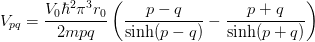
Vpq(p, q, m=1.0)[source]¶

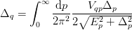
Integrated potential over angles that appears in the BCS s-wave gap equation:

$\Delta_{q} = \int_{0}^{\infty}\frac{\d{p}}{2\pi^2} \frac{V_{qp}\Delta_{p}}{2\sqrt{E_{p}^2 + \Delta_{p}^2}}$

Notes

$V_{pq} &= \frac{V_{0}\hbar^2\pi^3 r_{0}}{2 m p q}\left( \frac{p - q}{\sinh(p - q)} - \frac{p + q}{\sinh(p + q)} \right)$

Examples

>>> V = VPoschlTeller(r0=1)
>>> p = np.array([[0,1,2]])
>>> q = p.T
>>> V.Vpq(p,q)
array([[-6.57973627, -6.21059264, -5.25788171],
       [-6.21059264, -5.88551639, -5.03455853],
       [-5.25788171, -5.03455853, -4.4270986 ]])

class mmf.physics.potentials.separable.Separable(*varargin, **kwargs)[source]¶

Bases: mmf.objects.StateVars

Base class for separable potentials, including methods to compute their scattering properties: $a^{-1}$ and $r_{eff}$ are computed by potentials.ainv() and potentials.reff().

Separable(g=-1.0,
          m=1.0)

Notes

These potentials have the form:

$V(p,q) = gv(p)v(q)$

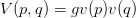
Our convention for normalization is that v(0) = 1. By default, the coupling constant is set to -1, so the potential is attractive. The form-factors $v(p)$ should be functions that decay for large momenta and are roughly constant for small momenta.

Attributes

State Variables:
`g`¶	Coupling constant
`m`¶	Mass. Set to reduced mass for two-body
Computed Variables:
`inf`¶	Infinite endpoint wrapped with a Decay subclass to encode the nature of the decay.
`p_c`[source]¶	List of typical/critical momenta. The points should be carefully inspected during integration etc.

Methods

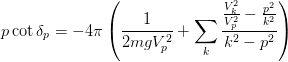
`ainv`([abs_tol, rel_tol])	Return the inverse s-wave scattering-length.
`all_items`()	Return a list [(name, obj)] of (name, object) pairs containing all items available.
`archive`(name)	Return a string representation that can be executed to restore the object.
`archive_1`([env])	Return (rep, args, imports).
`initialize`(**kwargs)	Calls `__init__()` passing all assigned attributes.
`items`([archive])	Return a list [(name, obj)] of (name, object) pairs where the
`k_cot_delta`(p2[, abs_tol, rel_tol])	Return the phase shift $p\cot\delta_p$ as a function of $p^2$ .
`reff`([abs_tol, rel_tol])	Return the s-wave effective range.
`resume`()	Resume calls to `__init__()` from `__setattr__()`,
`set_g`(ainv[, reff])	Set the coupling and Lambda to fix the scattering length
`suspend`()	Suspend calls to `__init__()` from
`v`(p)	Return the form factor.

Subclasses should call to add p_c to self.V

Methods

`ainv`([abs_tol, rel_tol])	Return the inverse s-wave scattering-length.
`all_items`()	Return a list [(name, obj)] of (name, object) pairs containing all items available.
`archive`(name)	Return a string representation that can be executed to restore the object.
`archive_1`([env])	Return (rep, args, imports).
`initialize`(**kwargs)	Calls `__init__()` passing all assigned attributes.
`items`([archive])	Return a list [(name, obj)] of (name, object) pairs where the
`k_cot_delta`(p2[, abs_tol, rel_tol])	Return the phase shift $p\cot\delta_p$ as a function of $p^2$ .
`reff`([abs_tol, rel_tol])	Return the s-wave effective range.
`resume`()	Resume calls to `__init__()` from `__setattr__()`,
`set_g`(ainv[, reff])	Set the coupling and Lambda to fix the scattering length
`suspend`()	Suspend calls to `__init__()` from
`v`(p)	Return the form factor.

__init__(*varargin, **kwargs)[source]¶: Subclasses should call to add p_c to self.V

ainv(abs_tol=1e-12, rel_tol=1e-12)[source]¶

Return the inverse s-wave scattering-length.

Notes

This is computed by

$a^{-1} = \frac{2\pi}{gmV_{0}^2} +\frac{2}{\pi V_{0}^2}\int_{0}^{\infty}\d{k}\;V_{k}^2$

k_cot_delta(p2, abs_tol=1e-12, rel_tol=1e-12)[source]¶: Return the phase shift $p\cot\delta_p$ as a function of $p^2$ .

$p\cot\delta_p = -4\pi\left(\frac{1}{2 m g V_p^2} + \sum_{k}\frac{\frac{V_k^2}{V_p^2} - \frac{p^2}{k^2}} {k^2 - p^2}\right)$

p_c[source]: List of typical/critical momenta. The points should be carefully inspected during integration etc.

reff(abs_tol=1e-12, rel_tol=1e-12)[source]¶

Return the s-wave effective range.

Notes

This is computed by:

$r_{\text{eff}} = \frac{8\pi \kappa}{gmV_{0}^2} - \frac{8}{\pi}\int_{0}^{\infty}\d{k} \frac{\frac{V_{k}^{2}}{V_{0}^{2}}\left(1-2k^2\kappa\right) -1 }{k^2}$

where $\kappa = \left.\diff{\ln V_{p}}{p^2}\right|_{p=0}$

set_g(ainv, reff=None)[source]¶: Set the coupling and Lambda to fix the scattering length and range.

v(p)[source]¶: Return the form factor.

class mmf.physics.potentials.separable.SharpCutoff(*varargin, **kwargs)[source]¶

Bases: mmf.physics.potentials.separable.Separable

Separable potential with a sharp momentum cutoff.

SharpCutoff(g=-1.0,
            m=1.0,
            Lambda=1.0)

Notes

$v(p) &= \theta(p - \Lambda),\\ \frac{1}{a} &= \frac{2\pi}{mg} + \frac{2\Lambda}{\pi},\\ r_{\text{eff}} &= \frac{4}{\pi\Lambda},\\ Pr_{\text{eff}}^{3} &= \frac{2}{3\pi\Lambda^3}.$

assume(L>0);assume(k>0);assume(p>0);additionally(L>k):
kcd:=(v)->-4*Pi*(1/2/m/g/v(k)**2 + int((v(p)**2/v(k)**2
                 - k^2/p^2)/(p^2-k^2)*p^2/2/Pi^2,p=0..infinity)):
v:=p->Heaviside(L-p):
ainv=-subs(k=0,kcd(v));
re=2*coeff(series(kcd(v),k,6),k,2);
P*re^3=coeff(series(kcd(v),k,6),k,4);

Examples

>>> V = SharpCutoff(Lambda=10.0)
>>> V.set_g(ainv=1.0, reff=0.1)
>>> V.ainv()                
1.00000000...
>>> V.reff()                
0.10000000...

Attributes

State Variables:
`g`¶	Coupling constant
`m`¶	Mass. Set to reduced mass for two-body
`Lambda`¶	Momentum cutoff
Computed Variables:
`inf`¶	Infinite endpoint wrapped with a Decay subclass to encode the nature of the decay.
`p_c`¶	List of typical/critical momenta. The points should be carefully inspected during integration etc.

Methods

`ainv`([abs_tol, rel_tol])	Return the inverse s-wave scattering-length.
`all_items`()	Return a list [(name, obj)] of (name, object) pairs containing all items available.
`archive`(name)	Return a string representation that can be executed to restore the object.
`archive_1`([env])	Return (rep, args, imports).
`initialize`(**kwargs)	Calls `__init__()` passing all assigned attributes.
`items`([archive])	Return a list [(name, obj)] of (name, object) pairs where the
`k_cot_delta`(p2[, abs_tol, rel_tol])	Return the phase shift $p\cot\delta_p$ as a function of $p^2$ .
`reff`([abs_tol, rel_tol])	Return the s-wave effective range.
`resume`()	Resume calls to `__init__()` from `__setattr__()`,
`set_g`(ainv[, reff])	Set the coupling to fix the scattering length.
`suspend`()	Suspend calls to `__init__()` from
`v`(p)

Subclasses should call to add p_c to self.V

Methods

`ainv`([abs_tol, rel_tol])	Return the inverse s-wave scattering-length.
`all_items`()	Return a list [(name, obj)] of (name, object) pairs containing all items available.
`archive`(name)	Return a string representation that can be executed to restore the object.
`archive_1`([env])	Return (rep, args, imports).
`initialize`(**kwargs)	Calls `__init__()` passing all assigned attributes.
`items`([archive])	Return a list [(name, obj)] of (name, object) pairs where the
`k_cot_delta`(p2[, abs_tol, rel_tol])	Return the phase shift $p\cot\delta_p$ as a function of $p^2$ .
`reff`([abs_tol, rel_tol])	Return the s-wave effective range.
`resume`()	Resume calls to `__init__()` from `__setattr__()`,
`set_g`(ainv[, reff])	Set the coupling to fix the scattering length.
`suspend`()	Suspend calls to `__init__()` from
`v`(p)

__init__(*varargin, **kwargs)¶: Subclasses should call to add p_c to self.V

set_g(ainv, reff=None)[source]¶

Set the coupling to fix the scattering length.

Notes

$\Lambda &= \frac{4}{r_{\text{eff}}\pi},\\ g &= m^{-1}\frac{2\pi}{a^{-1} - \frac{2\Lambda}{\pi}}.$

v(p)[source]¶

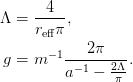
class mmf.physics.potentials.separable.SmoothCutoff(*varargin, **kwargs)[source]¶

Bases: mmf.physics.potentials.separable.Separable

Separable potential with a smooth momentum cutoff.

SmoothCutoff(g=-1.0,
             m=1.0,
             Lambda=1.0)

$v(p) &= e^{-\tfrac{\pi}{8}\frac{p^2}{\Lambda^2}},\\ \frac{1}{a} &= \frac{2\pi}{mg} + \frac{2\Lambda}{\pi},\\ r_{\text{eff}} &= \frac{1}{\Lambda} - \frac{\pi^2}{mg\Lambda^2},\\ Pr_{\text{eff}}^{3} &= \frac{\pi}{48\Lambda^3} - \frac{2\pi^3}{8g\Lambda^4}.$

assume(L>0);assume(k>0);assume(p>0);additionally(L>k):
kcd:=(v)->-4*Pi*(1/2/m/g/v(k)**2 + int((v(p)**2/v(k)**2
                 - k^2/p^2)/(p^2-k^2)*p^2/2/Pi^2,p=0..infinity)):
v:=p->exp(-Pi/8*p^2/L^2):
eqs:={ainv=-expand(simplify(eval(subs(k=0,kcd(v))))),
      re=2*expand(simplify(coeff(series(kcd(v),k,6),k,2)))};
P*re^3=coeff(series(kcd(v),k,6),k,4);
solve(eqs,[g,L]);

Examples

>>> a = 1.0
>>> V = SmoothCutoff(Lambda=10.0)
>>> V.set_g(ainv=1.0, reff=0.1)
>>> V.ainv()                
1.000000000...
>>> V.reff()                
0.100000000...

Attributes

State Variables:
`g`¶	Coupling constant
`m`¶	Mass. Set to reduced mass for two-body
`Lambda`¶	Momentum cutoff
Computed Variables:
`inf`¶	Infinite endpoint wrapped with a Decay subclass to encode the nature of the decay.
`p_c`¶	List of typical/critical momenta. The points should be carefully inspected during integration etc.

Methods

`ainv`([abs_tol, rel_tol])	Return the inverse s-wave scattering-length.
`all_items`()	Return a list [(name, obj)] of (name, object) pairs containing all items available.
`archive`(name)	Return a string representation that can be executed to restore the object.
`archive_1`([env])	Return (rep, args, imports).
`initialize`(**kwargs)	Calls `__init__()` passing all assigned attributes.
`items`([archive])	Return a list [(name, obj)] of (name, object) pairs where the
`k_cot_delta`(p2[, abs_tol, rel_tol])	Return the phase shift $p\cot\delta_p$ as a function of $p^2$ .
`reff`([abs_tol, rel_tol])	Return the s-wave effective range.
`resume`()	Resume calls to `__init__()` from `__setattr__()`,
`set_g`(ainv[, reff])	Set the coupling to fix the scattering length.
`suspend`()	Suspend calls to `__init__()` from
`v`(p)

Subclasses should call to add p_c to self.V

Methods

`ainv`([abs_tol, rel_tol])	Return the inverse s-wave scattering-length.
`all_items`()	Return a list [(name, obj)] of (name, object) pairs containing all items available.
`archive`(name)	Return a string representation that can be executed to restore the object.
`archive_1`([env])	Return (rep, args, imports).
`initialize`(**kwargs)	Calls `__init__()` passing all assigned attributes.
`items`([archive])	Return a list [(name, obj)] of (name, object) pairs where the
`k_cot_delta`(p2[, abs_tol, rel_tol])	Return the phase shift $p\cot\delta_p$ as a function of $p^2$ .
`reff`([abs_tol, rel_tol])	Return the s-wave effective range.
`resume`()	Resume calls to `__init__()` from `__setattr__()`,
`set_g`(ainv[, reff])	Set the coupling to fix the scattering length.
`suspend`()	Suspend calls to `__init__()` from
`v`(p)

__init__(*varargin, **kwargs)¶: Subclasses should call to add p_c to self.V

set_g(ainv, reff=None)[source]¶: Set the coupling to fix the scattering length.

$\Lambda &= \frac{1 + \sqrt{1-\frac{\pi}{2} \frac{r_{\text{eff}}}{a}}} {r_{\text{eff}}},\\ g &= m^{-1}\frac{2\pi}{a^{-1} - \frac{2\Lambda}{\sqrt{\pi}}}.$

v(p)[source]¶

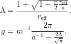
class mmf.physics.potentials.separable.Yamaguchi(*varargin, **kwargs)[source]¶

Bases: mmf.physics.potentials.separable.Separable

Separable Yamaguchi potential.

Yamaguchi(g=-1.0,
          m=1.0,
          Lambda=1.0)

$v(p) &= \frac{1}{\left(\frac{\pi p}{4\Lambda}\right)^2 + 1},\\ \frac{1}{a} &= \frac{2\pi}{mg} + \frac{2\Lambda}{\pi},\\ r_{\text{eff}} &= \frac{\pi}{4\Lambda} - \frac{\pi^3}{2mg\Lambda^2}\\ Pr_{\text{eff}}^{3} &= -\frac{\pi^5}{128 mg \Lambda^4}$

assume(L>0);assume(k>0);assume(p>0);additionally(L>k):
kcd:=(v)->-4*Pi*(1/2/m/g/v(k)**2 + int((v(p)**2/v(k)**2
                 - k^2/p^2)/(p^2-k^2)*p^2/2/Pi^2,p=0..infinity)):
v:=p->1/(1+(Pi*p/4/L)^2):
eqs:={ainv=-expand(simplify(eval(subs(k=0,kcd(v))))),
      re=2*expand(simplify(coeff(series(kcd(v),k,6),k,2)))};
P*re^3=coeff(series(kcd(v),k,6),k,4);
solve(eqs,[g,L]);
simplify(expand(rationalize(allvalues(solve(eqs,[g,L]))[1][1])));

Note: this has a closed effective range expansion with three terms.

Examples

>>> V = Yamaguchi(Lambda=10.0)
>>> V.set_g(ainv=1.0,reff=0.5)
>>> V.ainv()                
1.0...
>>> V.reff()                
0.499999...

Attributes

State Variables:
`g`¶	Coupling constant
`m`¶	Mass. Set to reduced mass for two-body
`Lambda`¶	Momentum cutoff
Computed Variables:
`inf`¶	Infinite endpoint wrapped with a Decay subclass to encode the nature of the decay.
`p_c`¶	List of typical/critical momenta. The points should be carefully inspected during integration etc.

Methods

`ainv`([abs_tol, rel_tol])	Return the inverse s-wave scattering-length.
`all_items`()	Return a list [(name, obj)] of (name, object) pairs containing all items available.
`archive`(name)	Return a string representation that can be executed to restore the object.
`archive_1`([env])	Return (rep, args, imports).
`initialize`(**kwargs)	Calls `__init__()` passing all assigned attributes.
`items`([archive])	Return a list [(name, obj)] of (name, object) pairs where the
`k_cot_delta`(p2[, abs_tol, rel_tol])	Return the phase shift $p\cot\delta_p$ as a function of $p^2$ .
`reff`([abs_tol, rel_tol])	Return the s-wave effective range.
`resume`()	Resume calls to `__init__()` from `__setattr__()`,
`set_g`(ainv[, reff])	Set the coupling and Lambda to fix the scattering length
`suspend`()	Suspend calls to `__init__()` from
`v`(p)

Subclasses should call to add p_c to self.V

Methods

`ainv`([abs_tol, rel_tol])	Return the inverse s-wave scattering-length.
`all_items`()	Return a list [(name, obj)] of (name, object) pairs containing all items available.
`archive`(name)	Return a string representation that can be executed to restore the object.
`archive_1`([env])	Return (rep, args, imports).
`initialize`(**kwargs)	Calls `__init__()` passing all assigned attributes.
`items`([archive])	Return a list [(name, obj)] of (name, object) pairs where the
`k_cot_delta`(p2[, abs_tol, rel_tol])	Return the phase shift $p\cot\delta_p$ as a function of $p^2$ .
`reff`([abs_tol, rel_tol])	Return the s-wave effective range.
`resume`()	Resume calls to `__init__()` from `__setattr__()`,
`set_g`(ainv[, reff])	Set the coupling and Lambda to fix the scattering length
`suspend`()	Suspend calls to `__init__()` from
`v`(p)

__init__(*varargin, **kwargs)¶: Subclasses should call to add p_c to self.V

set_g(ainv, reff=None)[source]¶: Set the coupling and Lambda to fix the scattering length and range.

$\Lambda = \frac{\pi}{8r_{\text{eff}}}\left( 3 + \sqrt{9-16\frac{r_{\text{eff}}}{a}}\right).$

v(p)[source]¶

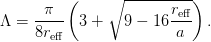
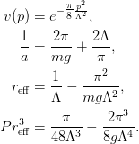
class mmf.physics.potentials.separable.EffectiveRange(*varargin, **kwargs)[source]¶

Bases: mmf.physics.potentials.separable.Separable

Separable Effective Range Interaction, completely determined by the scattering length and effective range.

EffectiveRange(g=-1.0,
               m=1.0,
               Lambda=1.0)

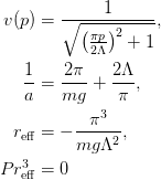
$v(p) &= \frac{1}{\sqrt{\left(\frac{\pi p}{2\Lambda}\right)^2 + 1}},\\ \frac{1}{a} &= \frac{2\pi}{mg} + \frac{2\Lambda}{\pi},\\ r_{\text{eff}} &= -\frac{\pi^3}{mg\Lambda^2},\\ Pr_{\text{eff}}^{3} &= 0$

assume(L>0);assume(k>0);assume(p>0);additionally(L>k):
kcd:=(v)->-4*Pi*(1/2/m/g/v(k)**2 + int((v(p)**2/v(k)**2
                 - k^2/p^2)/(p^2-k^2)*p^2/2/Pi^2,p=0..infinity)):
v:=p->1/sqrt((Pi*p/2/L)^2+1):
eqs:={ainv=-expand(simplify(eval(subs(k=0,kcd(v))))),
      re=2*expand(simplify(coeff(series(kcd(v),k,6),k,2)))};
P*re^3=coeff(series(kcd(v),k,6),k,4);
simplify(expand(rationalize(subs(allvalues(solve(eqs,[g,L]))[1][1],L)),symbolic));
solve(eqs,[g,L]);

Note that this as a closed effective range expansion stopping at the second term.

Examples

>>> V = EffectiveRange(Lambda=10.0)
>>> V.set_g(ainv=1.0,reff=0.5)
>>> V.ainv()                
1.000000...
>>> V.reff()                
0.500000...

Attributes

State Variables:
`g`¶	Coupling constant
`m`¶	Mass. Set to reduced mass for two-body
`Lambda`¶	Momentum cutoff
Computed Variables:
`inf`¶	Infinite endpoint wrapped with a Decay subclass to encode the nature of the decay.
`p_c`¶	List of typical/critical momenta. The points should be carefully inspected during integration etc.

Methods

`ainv`([abs_tol, rel_tol])	Return the inverse s-wave scattering-length.
`all_items`()	Return a list [(name, obj)] of (name, object) pairs containing all items available.
`archive`(name)	Return a string representation that can be executed to restore the object.
`archive_1`([env])	Return (rep, args, imports).
`initialize`(**kwargs)	Calls `__init__()` passing all assigned attributes.
`items`([archive])	Return a list [(name, obj)] of (name, object) pairs where the
`k_cot_delta`(p2[, abs_tol, rel_tol])	Return the phase shift $p\cot\delta_p$ as a function of $p^2$ .
`reff`([abs_tol, rel_tol])	Return the s-wave effective range.
`resume`()	Resume calls to `__init__()` from `__setattr__()`,
`set_g`(ainv[, reff])	Set the coupling and Lambda to fix the scattering length
`suspend`()	Suspend calls to `__init__()` from
`v`(p)

Subclasses should call to add p_c to self.V

Methods

`ainv`([abs_tol, rel_tol])	Return the inverse s-wave scattering-length.
`all_items`()	Return a list [(name, obj)] of (name, object) pairs containing all items available.
`archive`(name)	Return a string representation that can be executed to restore the object.
`archive_1`([env])	Return (rep, args, imports).
`initialize`(**kwargs)	Calls `__init__()` passing all assigned attributes.
`items`([archive])	Return a list [(name, obj)] of (name, object) pairs where the
`k_cot_delta`(p2[, abs_tol, rel_tol])	Return the phase shift $p\cot\delta_p$ as a function of $p^2$ .
`reff`([abs_tol, rel_tol])	Return the s-wave effective range.
`resume`()	Resume calls to `__init__()` from `__setattr__()`,
`set_g`(ainv[, reff])	Set the coupling and Lambda to fix the scattering length
`suspend`()	Suspend calls to `__init__()` from
`v`(p)

__init__(*varargin, **kwargs)¶: Subclasses should call to add p_c to self.V

set_g(ainv, reff=None)[source]¶: Set the coupling and Lambda to fix the scattering length and range.

$\Lambda &= \frac{1+\sqrt{1 - \frac{2r_{\text{eff}}}{a}}} {2r_{0}/\pi},\\ g &= \frac{4\pi}{a^{-1} - \frac{\Lambda}{\sqrt{\pi}}}.$

v(p)[source]¶

Navigation

This Page

Quick search

mmf.physics.potentials.separable¶

Navigation

`mmf.physics.potentials.separable`¶