`mmf.math.integrate.acceleration`¶

levin(s[, type, k0, degree, ds]) Return the triangular acceleration table a for n terms of

This module provides some techniques for sequence acceleration.

Most of the theory and notation follows D. Laurie’s discussion in Appendix A. of [R4]. The general model is that the sequence has the form:

$s_k = s + \sum_{j=1}^{m} c_{j} \phi_{k,j} + \eta_k$

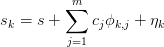
where $s$ is the converged result, $\phi_{k,j}$ is some set of known residual dependencies with unknown coefficients $c_j$ and $\eta_k$ is a residual that will be taken to be negligible [R3].

The acceleration will be summarized in a table of coefficients $s_{k,n}$ as follows:

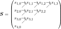
$\newcommand{\myarrows}{\;\mathllap{\rightarrow\kern-1.2em \lower0.6em\hbox{\ensuremath{\nearrow}}}} \mat{S} = \begin{pmatrix} s_{1,0} & \myarrows s_{1,1} & \myarrows s_{1,2} & \myarrows s_{1,3}\\ s_{2,0} & \myarrows s_{2,1} & \myarrows s_{2,2}\\ s_{3,0} & \myarrows s_{3,1}\\ s_{4,0} \end{pmatrix}$

where the arrows show the dependencies: Each term $s_{n,k}$ is a function of the terms $\{s_{n}, s_{n+1}, \cdots s_{n+k}\}$ . The first column is thus the original sequence.

Linear Accelerations¶

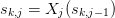Here we consider linear sequence transformations $X$ such that $X(as_{k} + bt_{k}) = aX(s_{k}) + bX(t_{k})$ . In particular, we consider each column of $\mat{S}$ to be a linear transformation of the previous column: $s_{k,j} = X_{j}(s_{k,j-1})$ . In this case, we may provide an explicit construction using n terms that eliminates the first n residuals by demanding:

(1) $\begin{aligned} s_{k+\delta} &= s_{k,n} + \sum_{j=1}^{n}c_{j}\phi_{k+\delta,j}, & \delta &\in[0,1,\cdots,n]. \end{aligned}$

This defines the entry $s_{k,n}$ in terms of the original elements of the sequence below and to the left by defining $n + 1$ equations for the $n+1$ unknowns $\{s_{k,n}, c_{1,\cdots,n}\}$ . Note that for each $s_{n,k}$ , the set of coefficients $c_{j}$ is different because this is not the original sequence (for example, we have truncated and ignored the error terms $\eta_{k}$ ).

Naively, one may directly solve these systems of equations for each of entries $s_{k,n}$ , but this takes $\order(n^5)$ operations. There is a general procedure called the “E-algorithm” that reduces this to $\order(n^3)$ which we now present. This is implemented by e_algorithm(). For special forms of the residuals $\phi_{k,j}$ specialized methods exist which are often much faster. Some of these are described later.

Note

For linear models, one should obtain convergence either proceeding down or to the right, but the key feature is that the convergence of the rows to the right should be much faster: this indicates that the underlying model is good. If the rows do not converge much faster than the columns, one should consider a different acceleration technique.

General E-Algorithm¶

As we discussed above, each successive column of S may be expressed in terms of this as an affine combination of the previous two entries $s_{k,j-1}$ and $s_{k+1,j-1}$ :

$\begin{aligned} s_{k,j} &= f_{k,j}s_{k,j-1} + (1-f_{k,j})s_{k+1, j-1}\\ &= s_{k+1, j-1} + \frac{r_{k,j}}{1-r_{k,j}}(s_{k+1,j-1}-s_{k,j-1}) \end{aligned}$

(The affinity is required to preserve the linearity, for example, so that $s_{:,j} + x$ and $s_{:,j+1} + x$ converge to the same value $s + x$ .)

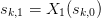
Start with the original sequence $s_{k,0}$ as the first column of $\mat{S}$ . Consider this, along with the new sequence $s_{k,1} = X_{1}(s_{k,0})$ and the sequence of residuals $\phi_{k,1}$ . The transformation $X$ can be represented as a matrix:

$\mat{X}_{1} = \begin{pmatrix} f_{1,1} & 1 - f_{1,1}\\ & f_{2,1} & 1 - f_{2,1}\\ & & \ddots & \ddots \end{pmatrix}$

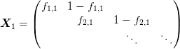
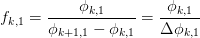
Equations (1) for $n=1$ are then satisfied if $X_{1}(\phi_{k,1}) = 0$ which defines the coefficients:

$f_{k,1} = \frac{\phi_{k,1}}{\phi_{k+1,1} - \phi_{k,1}} = \frac{\phi_{k,1}}{\Delta\phi_{k,1}}$

The E-algorithm is then to apply this transformation $X_{1}$ to the rest of the columns of $\phi_{k,j}$ to obtain a new set of residuals (the first column having been annihilated). Now treat $s_{k,1}$ as the new original sequence and repeat the process. This is implemented by e_algorithm(). In certain special cases, one can directly derive formula for the coefficients $r_{k,j}$ . The table $\mat{S}$ can them be directly constructed. This is done in direct_algorithm().

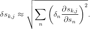
To estimate the error-sensitivity, we consider each entry $s_{k,j}(s_{k}, s_{k+1}, \cdots, s_j)$ to be a function of the original sequence entries. Given errors in the input $s_j \pm \delta_j$ , an estimate of the error in the result is

$\delta s_{k,j} \approx \sqrt{ \sum_{n} \left(\delta_n\pdiff{s_{k,j}}{s_n}\right)^2}.$

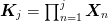For linear algorithms, this is easy to compute since $s_{k,j} = \left[\mat{K}_{j}\cdot \vect{s}\right]_k$ where $\mat{K}_{j} = \prod_{n=1}^{j}\mat{X}_{n}$ . The squares of the errors $(\delta s_{k,j})^2$ will be the diagonals of the matrix $\mat{K}\cdot\diag{\delta_n^2}\cdot\mat{K}^{T}$ .

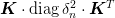For some of the faster specialized algorithms, it is a bit cumbersome to compute this exactly, so we directly propagate the errors as either

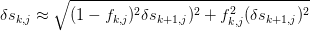
$\delta s_{k,j} \approx \sqrt{(1-f_{k,j})^2\delta s_{k+1,j})^2 + f_{k,j}^2(\delta s_{k+1,j})^2}$

or

$\delta s_{k,j} \approx \abs{1-f_{k,j}}\delta s_{k+1,j} + \abs{f_{k,j}}\delta s_{k+1,j})$

This will overestimate the errors as cancellations that occur at various stages are not taken into account, but in practise, this is not very significant.

Richardson Extrapolation¶

The Richardson extrapolation method considers models of the form

(2) $\phi_{k,j} = h_k^{P_j}$

These most typically arise in problems such as differentiation, integration, or discretization where there is a step-size $h_k$ that is decreased at successive stages. The most general model (2) requires the full E-algorithm, but there are several special cases that admit analytic solutions:

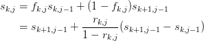
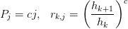
Geometric progression of step sizes with constant r:

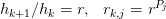
$\begin{aligned} h_{k+1}/h_{k} &= r, & r_{k,j} &= r^{P_j} \end{aligned}$
Arithmetic progression of exponents:

$\begin{aligned} P_{j} &= c j, & r_{k,j} &= \left(\frac{h_{k+1}}{h_{k}}\right)^{c} \end{aligned}$

Modified Salzer’s Extrapolation¶

The modified Salzer’s extrapolation is based on a model of the form

$\phi_{k,j} = \frac{\psi_k}{(k+k_0)^{j-1}}.$

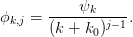
This provides another efficient method which can be derived by dividing (1) by $\psi_{k+\delta}$ :

$\begin{aligned} \frac{s_{k+\delta}}{\psi_{k+\delta}} &= \frac{s_{k,n}}{\psi_{k+\delta}} + \sum_{j=0}^{n-1} \frac{c_{j+1}}{(k+\delta+k_{0})^j}, & \delta \in [0,1,\cdots,n]. \end{aligned}$

From this we can construct the solution in terms of the divided difference operators $D^{n}$ : at $\delta=0$ which acts as a difference of the sequence $s_k$ as a function of $t_k = (k + k_0)^{-1}$ . The idea here is that the sum on the right is a polynomial of order $n-1$ in t_k, and hence will be annihilated by the n th difference operator at $\delta=0$ .

$D^0 s_k &= s_k\\ D^{n} s_k &= \frac{D^{n-1} s_{k+1} - D^{n-1} s_{k}}{t_{k+n} - t_k}\\ s_{k,n} &= \frac{D^{n}\left(\frac{s_k}{\psi_k}\right)} {D^{n}\left(\frac{1}{\psi_k}\right)}$

Semi-linear Accelerations¶

The previous linear acceleration techniques are fairly robust, and one can generally prove that if the original sequence converges, then the accelerated sequence will also converge to the same limit. However, to obtain convergence, one must put good inputs into the model (1).

Perhaps the most famous of these methods are those due to Levin. These are generalizations of the Salzer expansion where the function $\psi_k$ is expressed in terms of the residuals $a_k = s_{k+1} - s_k$ of the sequence (as opposed to linear methods where $\psi_k$ is determined a priori independently of the actual sequence). Semi-linear methods often work well, even if no a priori information about the sequence is know, however, they are also more difficult to characterize. (For example, even if the transformation is exact for two sequences, it may not be exact for them sum as the transformations are not completely linear.)

To understand where the Levin transformation works, note that $a_k \sim$

The three most common Levin accelerations are:

T: $\psi_k = a_k$

U: $\psi_k = (k + k_0)a_k$

W: $\psi_k = \frac{a_k^2}{a_{k+1} - a_{k}}$

Notes and References¶

[R3]

Determining the form of $\phi_{k,j}$ is somewhat of an art. It is not just sufficient to choose an accurate sequence: the residual $\eta_{k}$ that remains after summing m terms must really be negligible. For example, consider $s = \sum_{k=1}^{\infty} k^{\alpha}$ with partial sums $s_k$ . From the residual, one might be tempted to use $\phi_{k,j} = {k+j}^{\alpha}$ which will ultimately be exact. However, after summing only n terms, the residual will still be $\eta_{k} = \sum_{j=2m}^{\infty}{k+j}^{\alpha} \approx \order[(2m)^{\alpha+1}]$ which is certainly not negligible if the series needs convergence acceleration!

Instead, one must find a good set of approximation that fall off sufficiently rapidly which is why these types of sequences work well with Salzar’s modified algorithm.

[R4]	F. Bornemann, D. Laurie, S. Wagon, and J. Waldvogel, The SIAM 100-Digit Challenge: A Study in High-Accuracy Numerical Computing, SIAM, 2004.

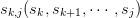
mmf.math.integrate.acceleration.levin(s, type='u', k0=0, degree=None, ds=None)[source]¶

Return the triangular acceleration table a for n terms of the sequence s[k] using the Levin transformation type.

Parameters :

s : 1-d array of length n

s[k] should be the k’th term in the sequence.

type : ‘t’, ‘u’, or ‘w’

Type ‘u’ is typically the most generally useful as it works whenever type ‘t’ works, however, ‘t’ works well for sequences $s_k \sim r^k$ and usually requires one less term, so for these types of sequences, it should be used to reduce roundoff error. For types ‘t’ and ‘u’ the returned table acceleration table a is (n-1 x n-1). For type w, the table is (n-2 x n-2).

k0 : float

Constant for the ‘u’ transform.

degree : int

Degree of extrapolation to use to determine last difference a_k

ds : None or float or 1-d array of length n

This should be an estimate of the errors in the terms of the sequence. If it is a single number, it is interpreted as the relative error in the terms, otherwise it is taken to be the array of absolute errors.

If it is not None, then the error estimate array dS will also be returned.

Returns :

S : array (n x n)

Triangular acceleration array. The rows S[k,:] should converge faster than the columns S[:,n], otherwise the model should not be trusted. Without round-off error, S[0,-1] would be the best estimate, but at some point, round-off error becomes significant.

dS : array (n x n)

If ds is provided and not None, then this array of error estimates will also be returned.

Table Of Contents

Previous topic

Next topic

This Page

`mmf.math.integrate.acceleration`¶