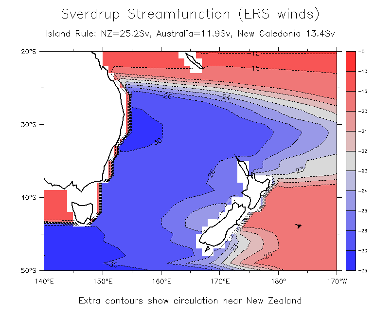
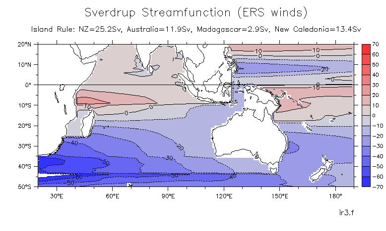
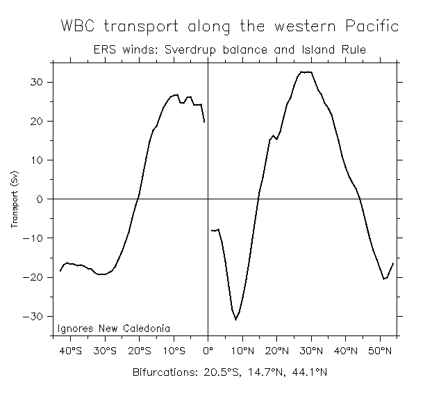
Island Rule (ERS winds)
Island Rule (ERS winds)
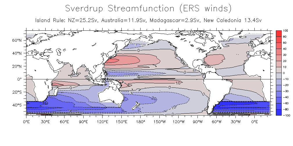
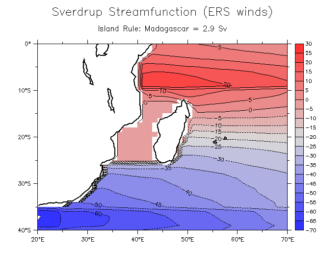
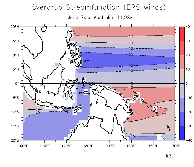
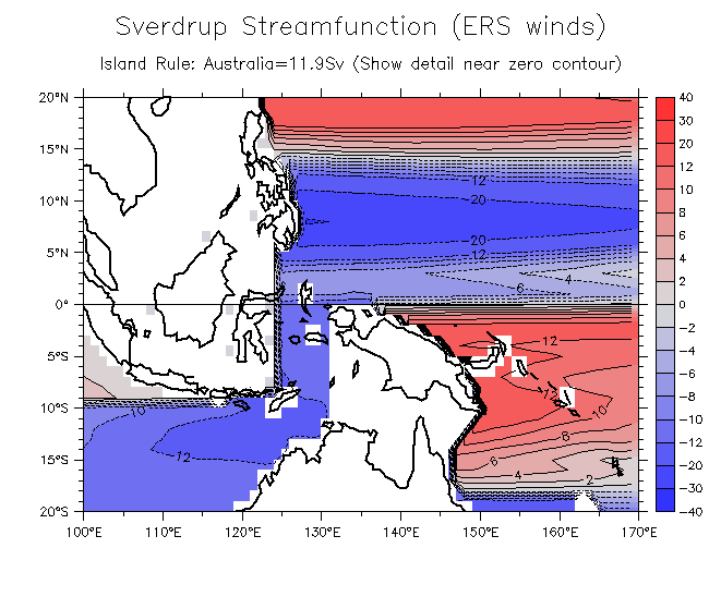
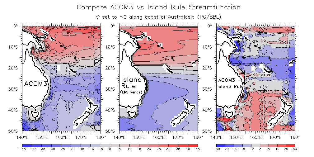
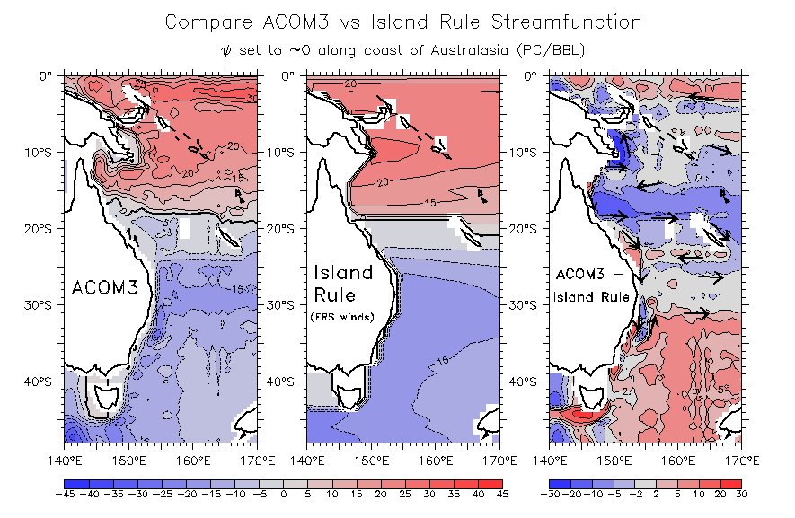
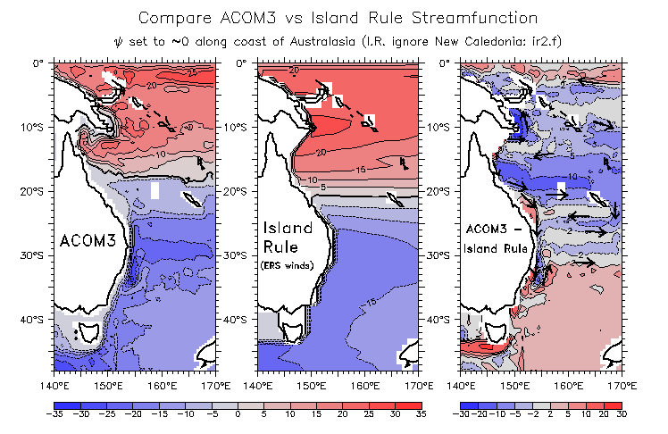
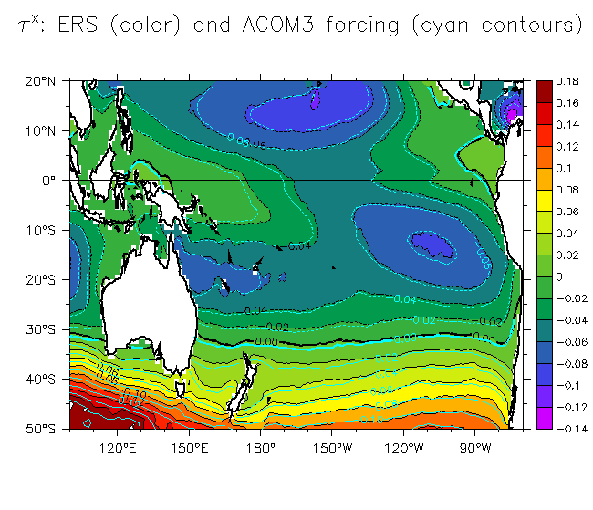
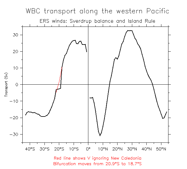
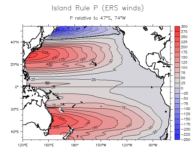
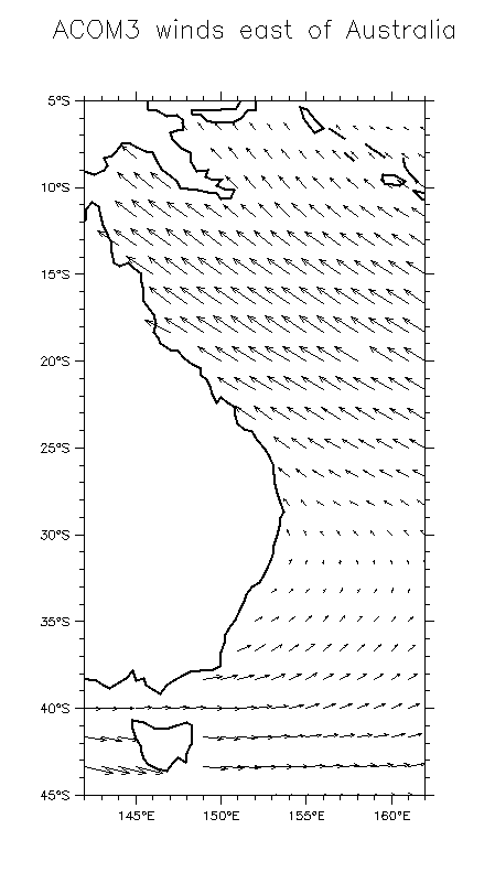
The Godfrey (1989) "Island Rule" calculation was repeated with ERS winds.
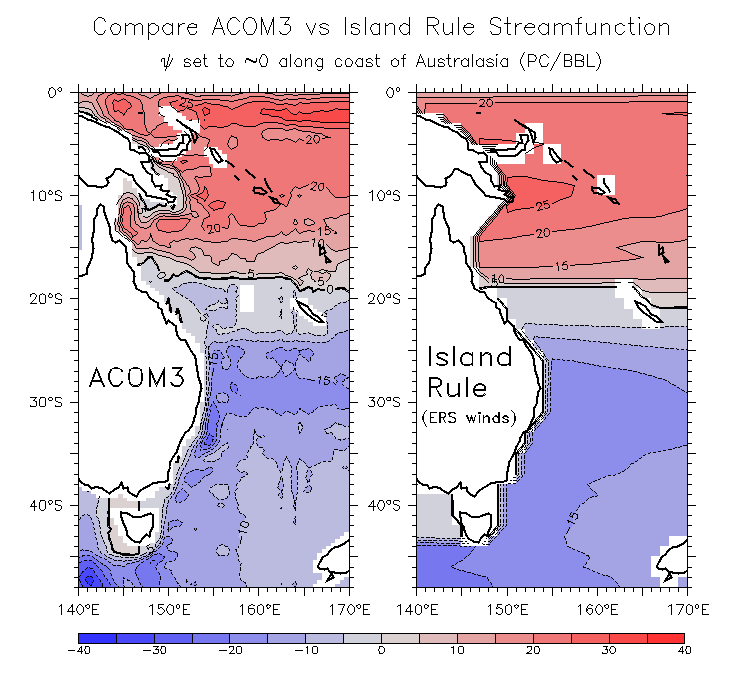
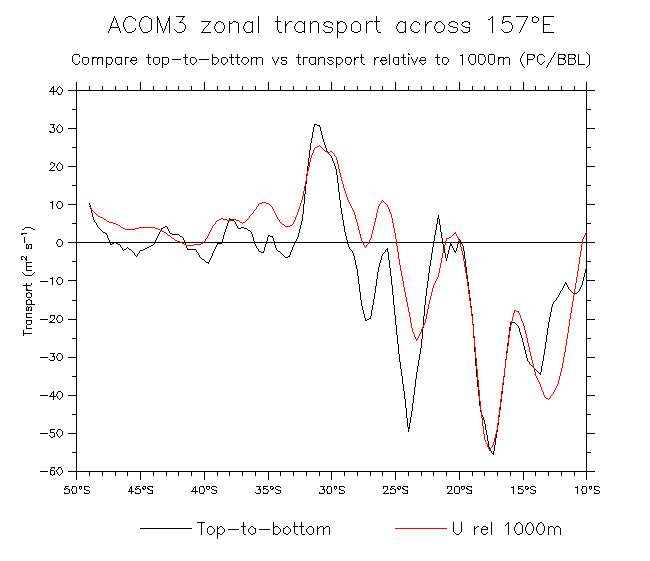
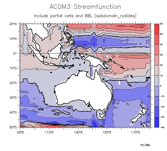
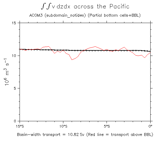
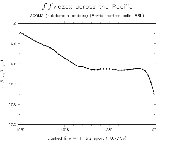
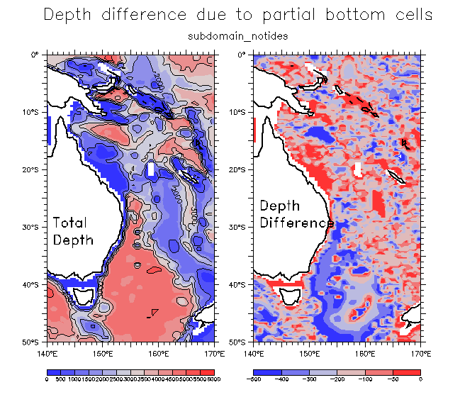
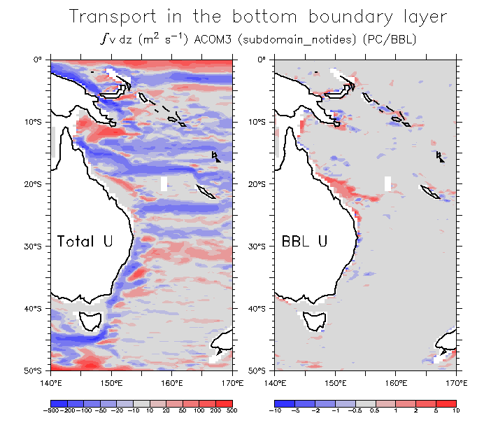
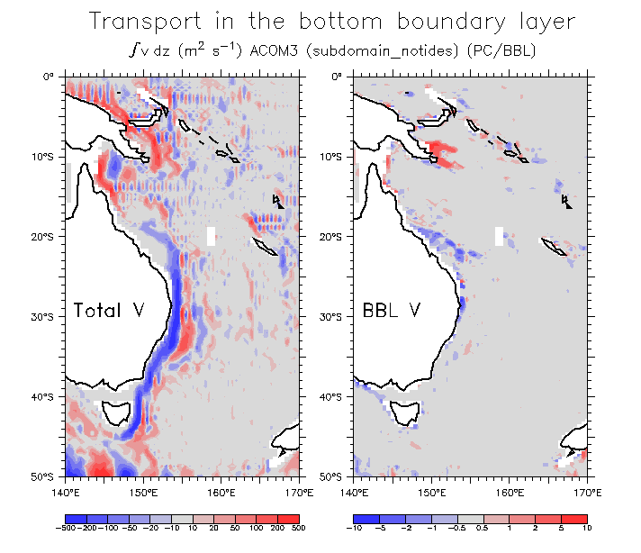
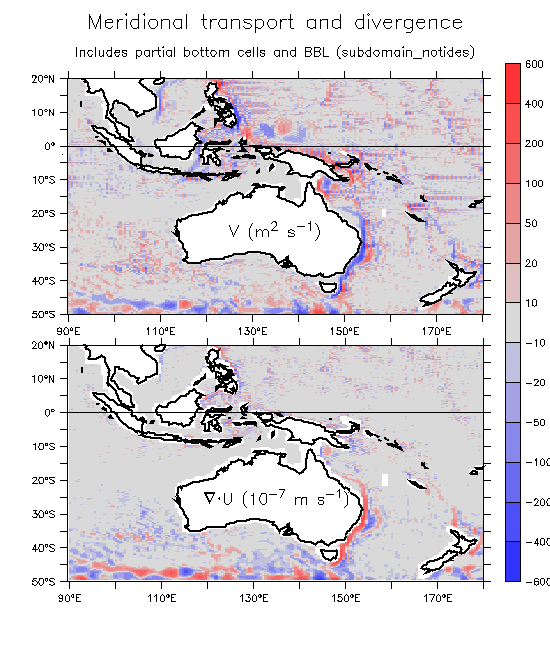
Note: in the course of this work two aspects of the ACOM3 runs were found that affect the results: The MOM model has "partial bottom cells", which make the grid nonhomogeneous, and also has a 50m-thick bottom boundary layer. Taking those thicknesses properly into account is essential to getting the top-to-bottom transport right. See Figs 4.5 for some details. Many plots on this page include streamfunctions or other transport measures from ACOM3. Not all of them have been redone to correct the vertical integrals. To check, look for the notation "PC/BBL" in the lower left corner of each plot (or in the main title).
- Global streamfunction
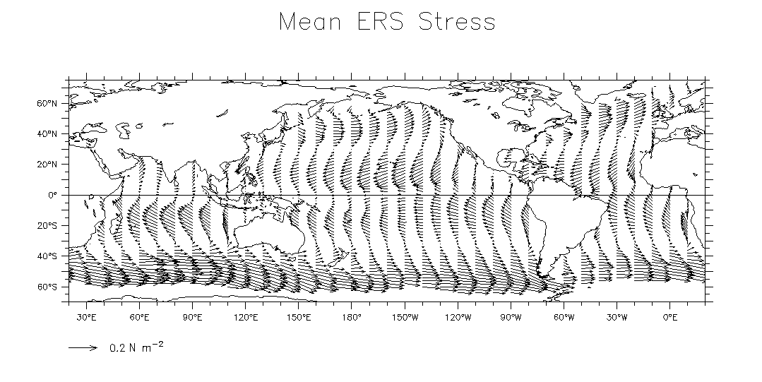
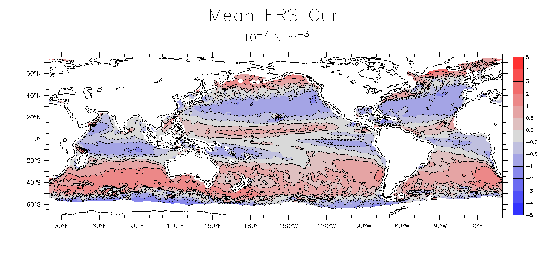
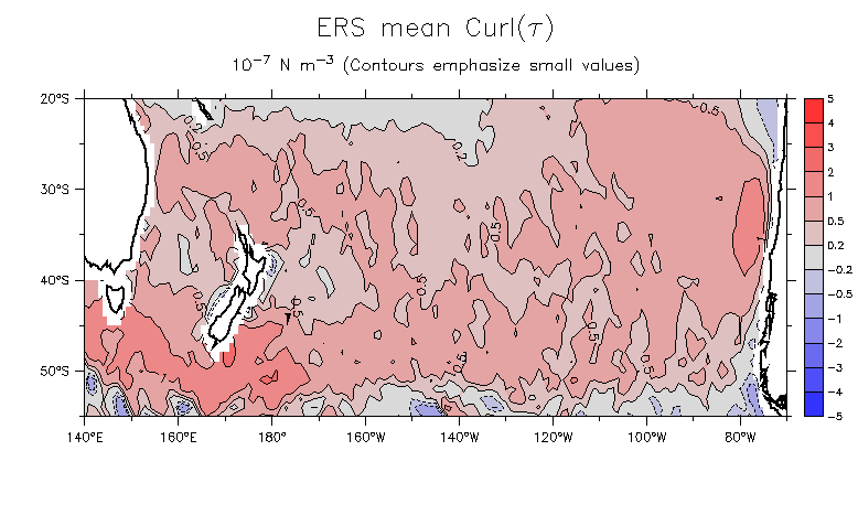
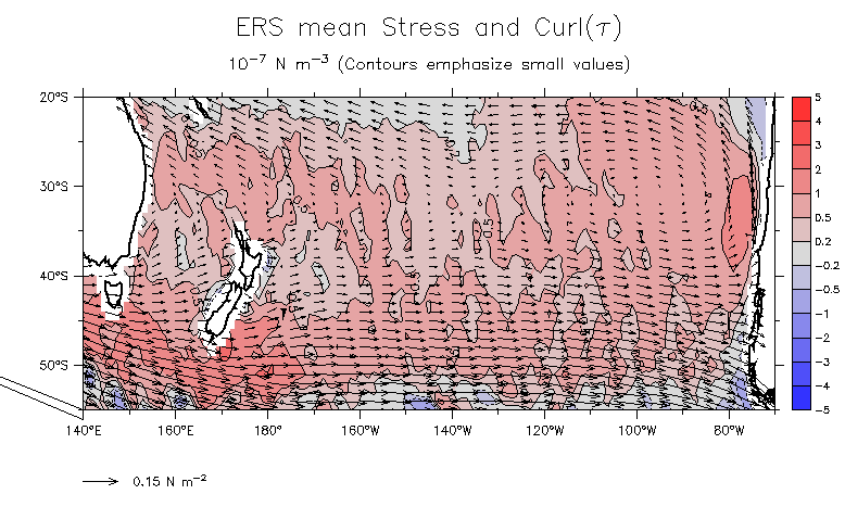
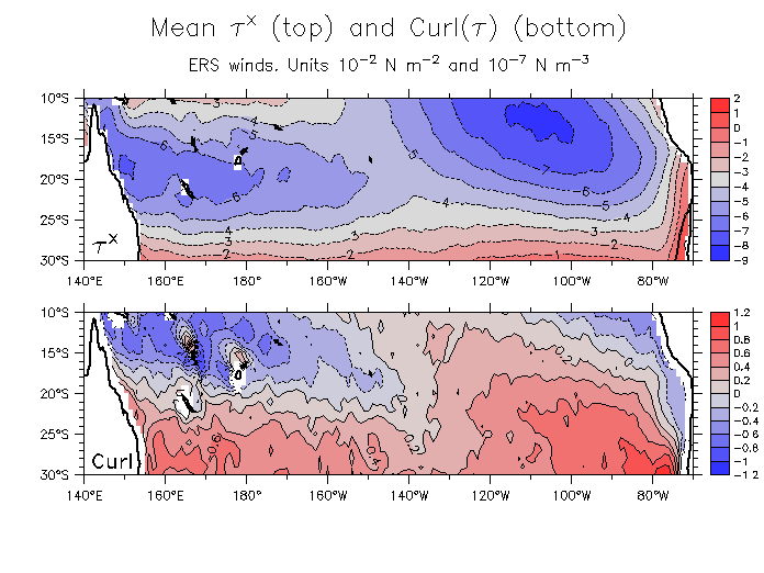
- Winds and curl: Stress 1 Stress 2 Curl Stress and curl
- Sverdrup streamfunction: Global
Details:
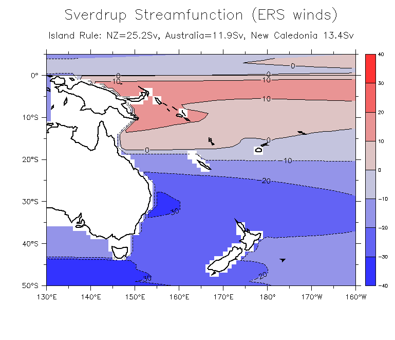
- Southwest Pacific
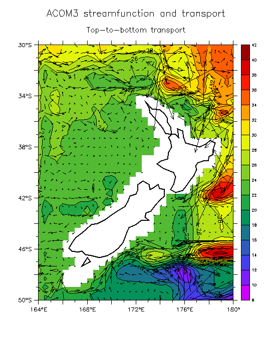
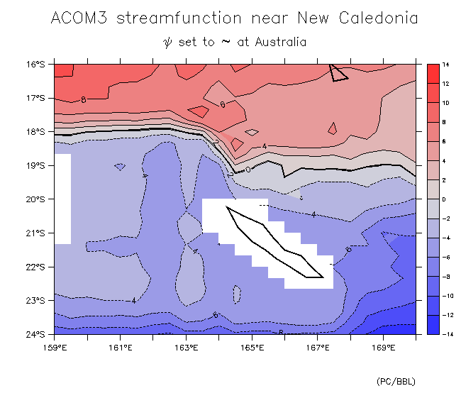
- NZ region (Curl for this integration Overlay Tau) Compare ACOM3 streamfunction
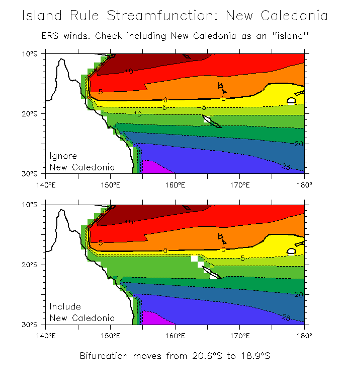
- Compare streamfunction ignoring New Caledonia vs treating it as an "island":
New Caledonia comparison (Detail) (Also see plots of P in 2.2 below)
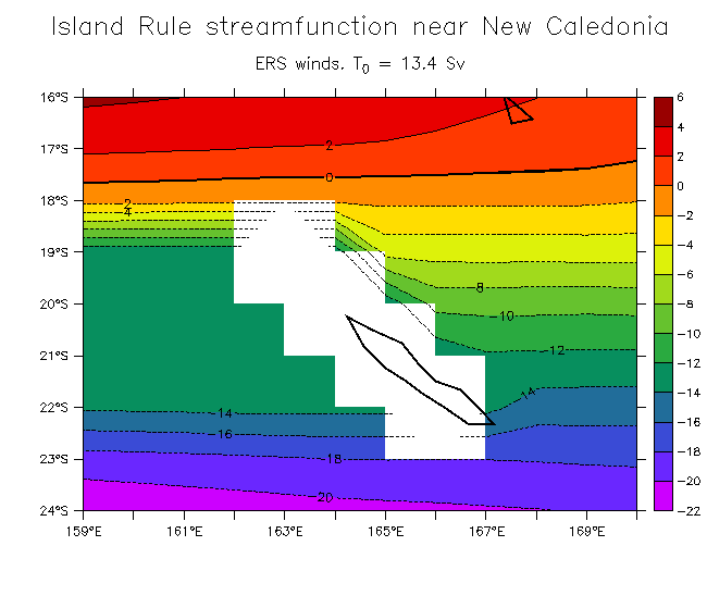
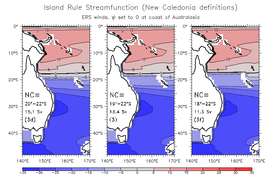
Check various definitions of New Caledonia size
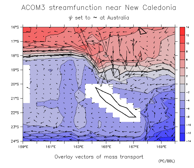
ACOM3 streamfunction: NC detail Add vectors (note 2dx oscillation NE of NC)
- Madagascar region
- Indian Ocean region
- Throughflow region
(more contours)
- Circulation around Australia
For ERS winds, the throughflow makes little difference in the SEC bifurcation latitude (unlike G89 H&R winds, see Fig 1.2h below).
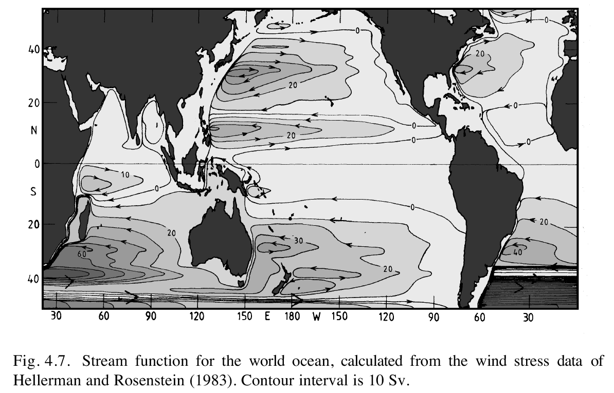
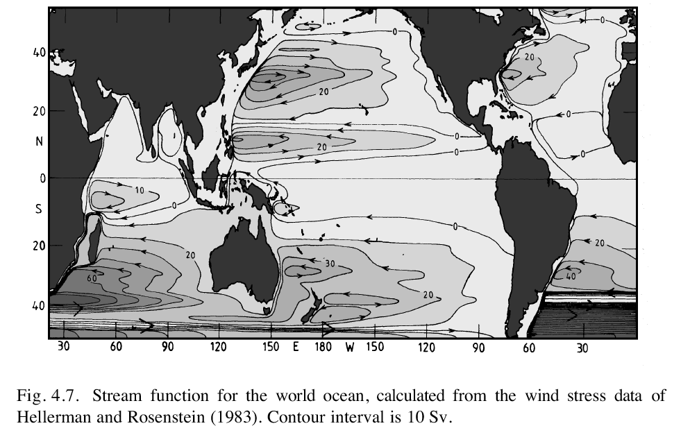
- Compare Godfrey (1989): (large) (small) (Fig 4.7 of Tomczak and Godfrey "Regional Oceanography")
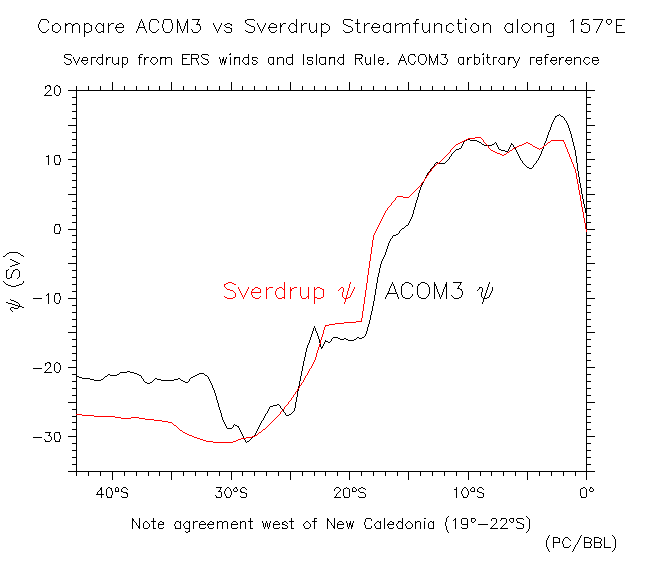
- Compare Sverdrup vs ACOM3 streamfunction east of Australasia: Maps (Extended) Along 157°E Difference maps (Ignore New Caledonia) Zonal and meridional components: ACOM3 Island Rule
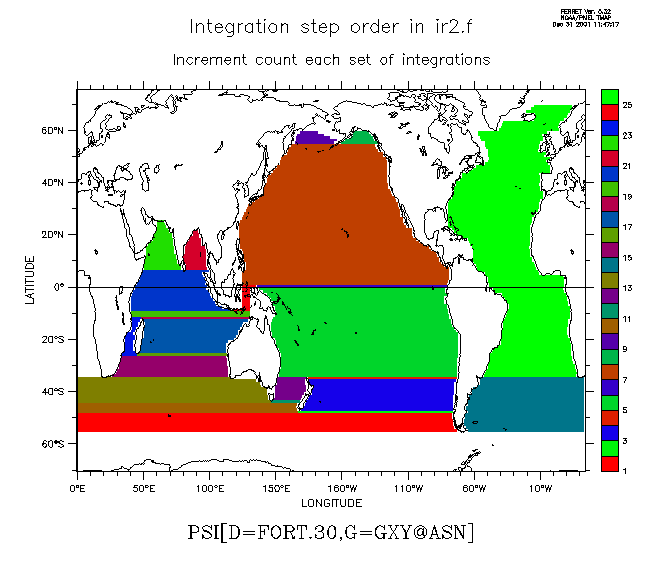
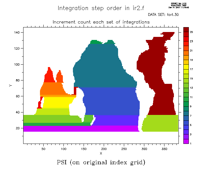
- Some checks of the code in progress: (By step): xy grid Index grid. (By sets): xy grid Index grid
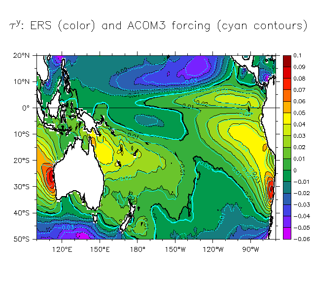
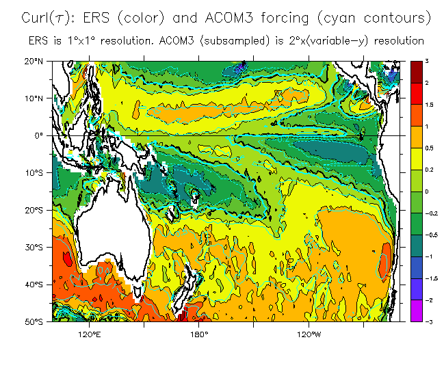
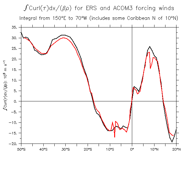
- Check ERS winds vs ACOM3 forcing winds: Taux Tauy Curl Zonally-integrated curl
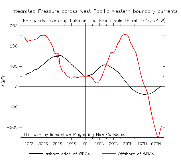
- Pressure across Pacific western boundary currents. A la Godfrey 89 (ms) Fig 7b.
- P across Pacific WBCs Transports (First cut: Ignores new Caledonia)
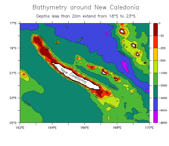
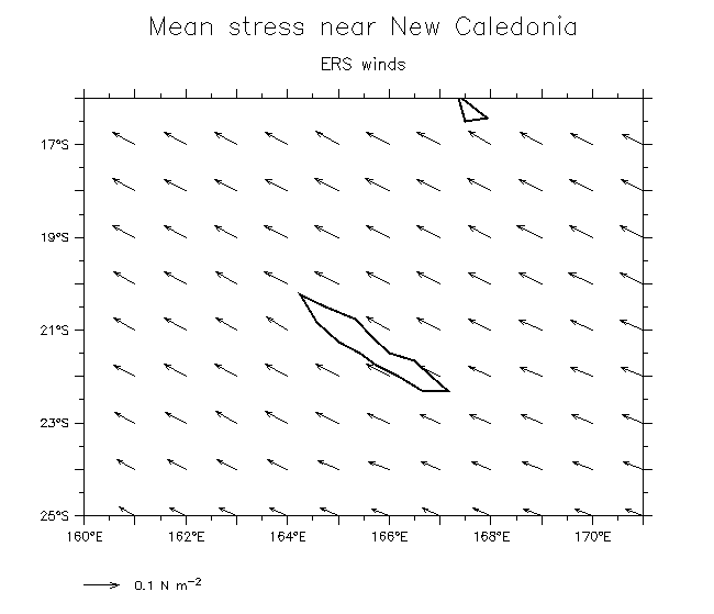
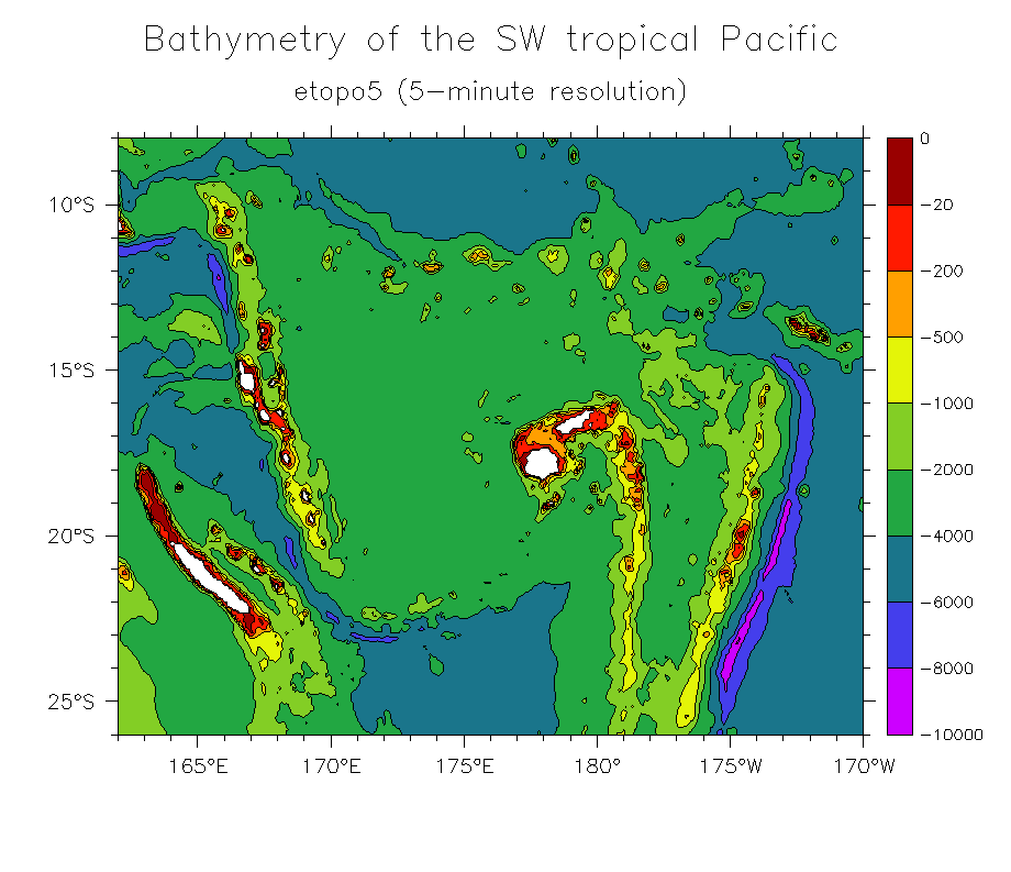
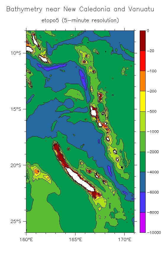
- Does New Caledonia matter?
- NC Bathymetry Tau near NC Taux and Curl (30°S-10°S)
- P across Pacific WBCs Transports
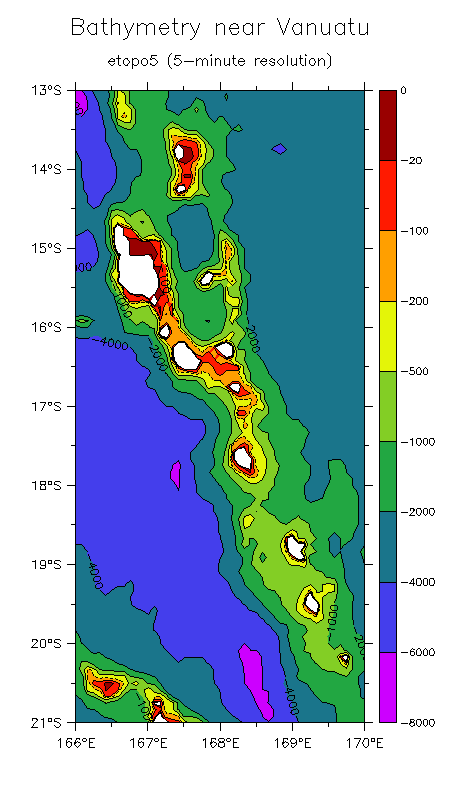
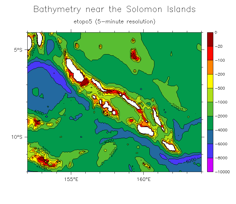
- More bathymetry: SW Pacific NC and Vanuatu Vanuatu Solomon Is. Solomon Is.
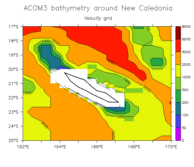
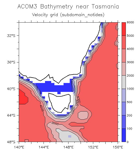
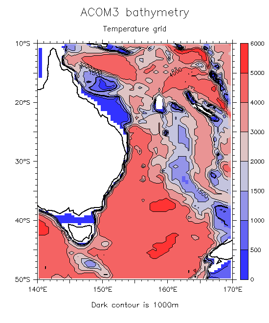
- ACOM3 bathymetry near New Caledonia Tasmania Coast of Australia
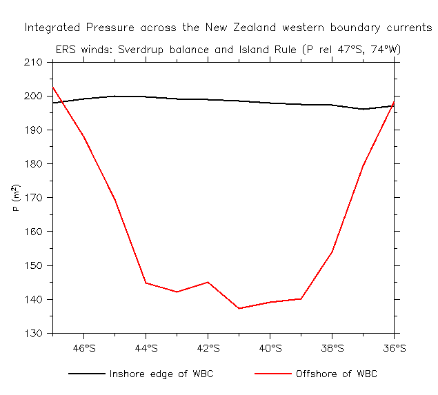
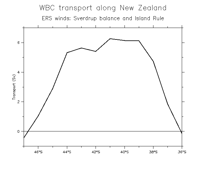
- The WBC along the east coast of New Zealand: P across WBC WBC transport
- Basinwide P(x,y)
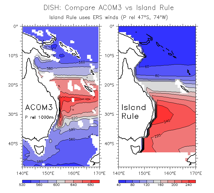
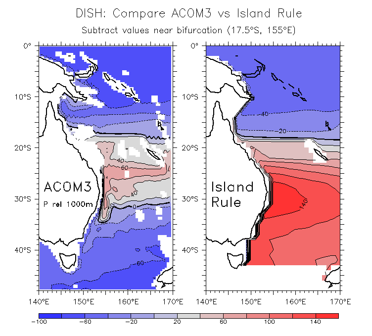
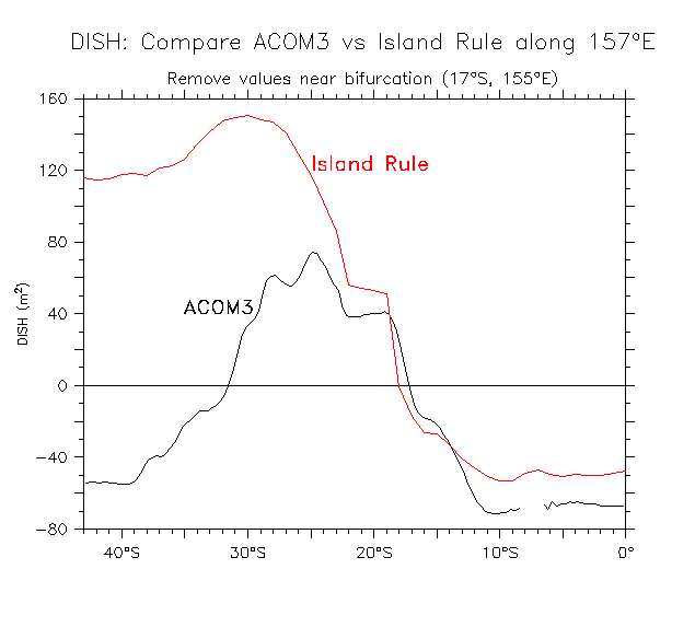
- Compare ACOM3 and Sverdrup DISH (rel 1000m) east of Australia:
- Original reference Adjusted reference Along 157°E
- Although the Sverdrup and ACOM3 streamfunctions are similar (Figs 1.3 above), the corresponding DISH patterns are not.
- Sverdrup DISH is maximum along 30°S, whereas the ACOM3 DISH max is along 25°S, among other systematic differences.
- The pattern of ACOM3 DISH is quite different from the top-to-bottom ACOM3 streamfunction: ACOM3 DISH vs Streamfunction (which is similar to the difference between ACOM3 and Sverdrup DISH)
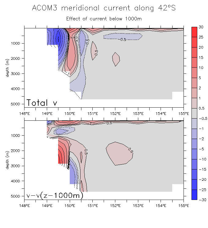
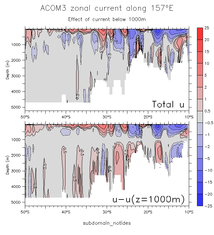
- The reason is signficant deep currents and pressure gradients in ACOM3:
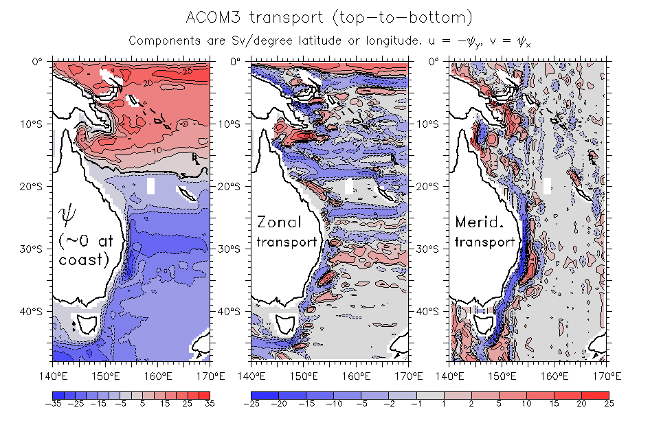
v along 42°S, u along 157°E, Transport along 157°E
- This will make it tricky to compare ACOM3 and Sverdrup pressures. Choosing a deeper reference level has the problem of topography, which is starting to intrude even at 1000m: ACOM3 bathymetry in the SW Pacific
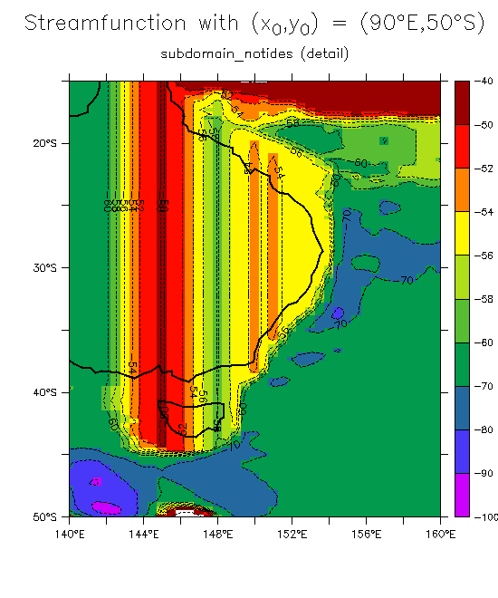
- ACOM3 streamfunction details:
(See also plots under 1.3 above)
- ACOM3 streamfunction
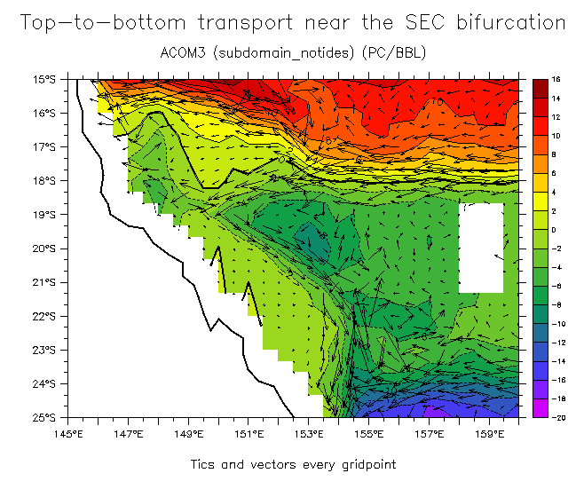
- Contours: 90°E-180°, 50°S-20°N Around Australia Detail near SEC bifurcation (With bathymetry)
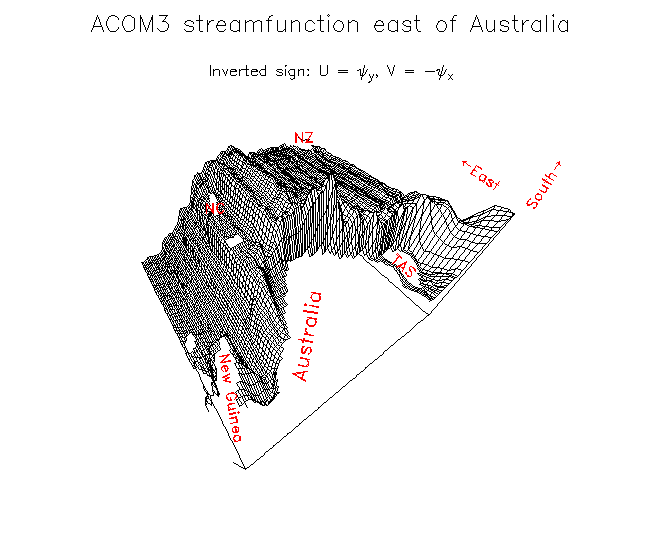
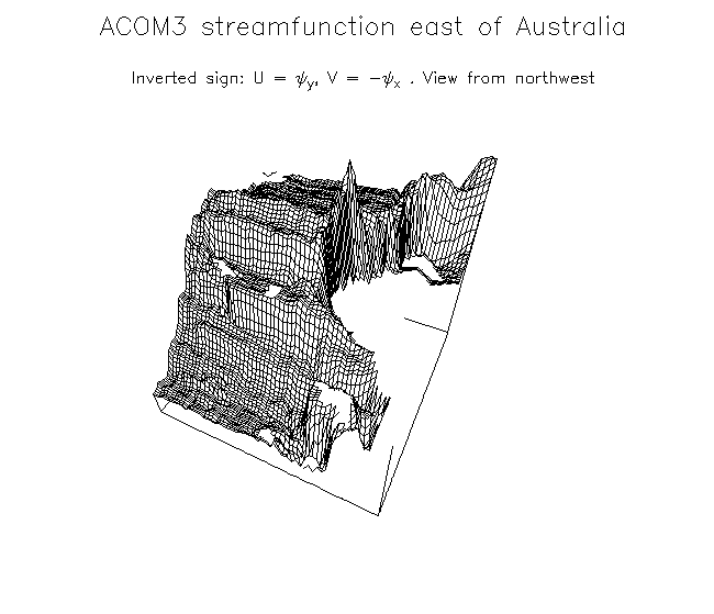
- Wireframe plots: View 1 View 2
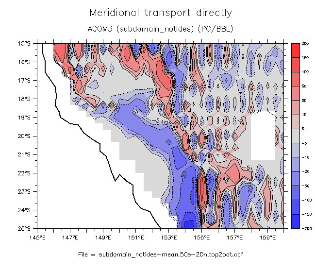
- Meridional transport near bifurcation: Direct vertical integration (2dx wave problems) From V=d(Psi)/dx (artifacts from 50°S)
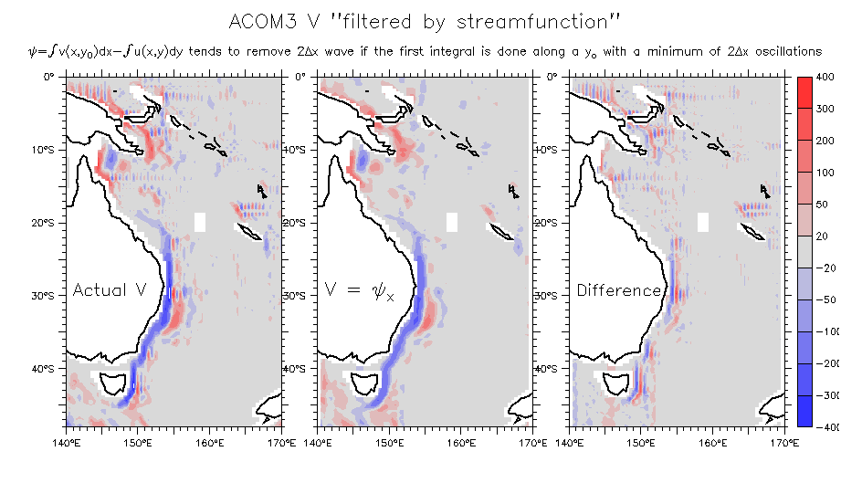
- Filtering by streamfunction (2dx wave)
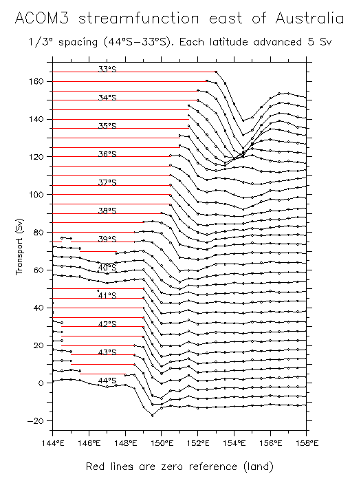
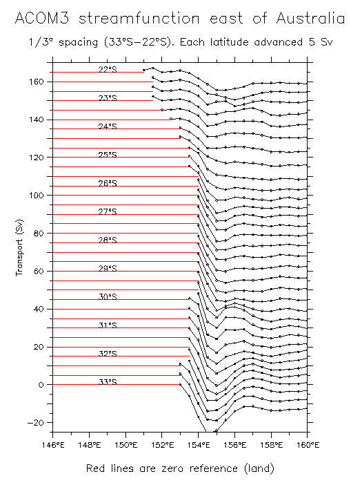
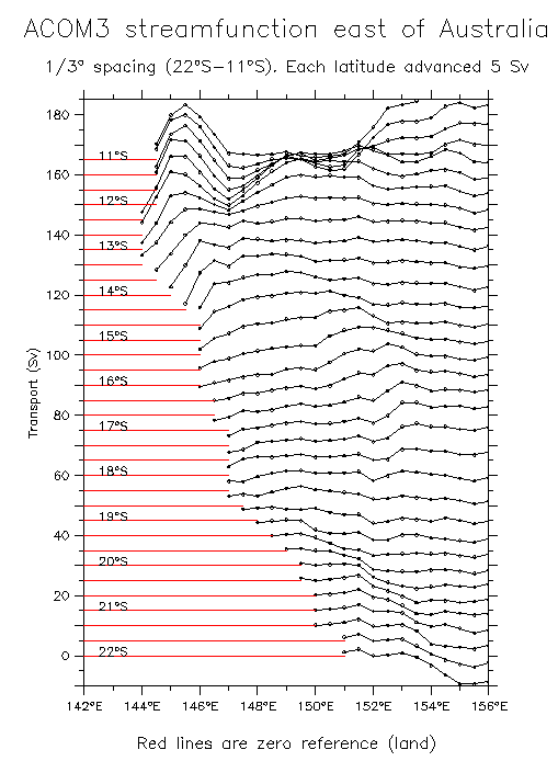
- Lineplots east of Australia: 44°S-33°S 33°S-22°S 22°S-11°S
[Old ones (no partial bottom cells): 44°S-33°S 33°S-22°S 22°S-11°S ]
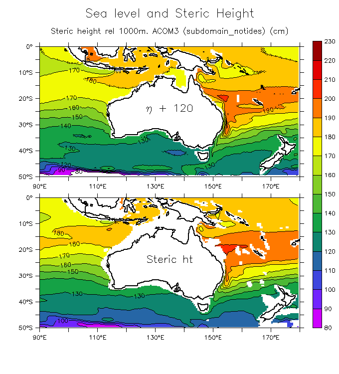
- ACOM3 absolute steric ht: Sea level and steric ht Absolute steric ht at 1000m
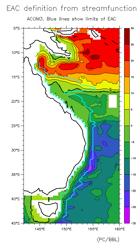
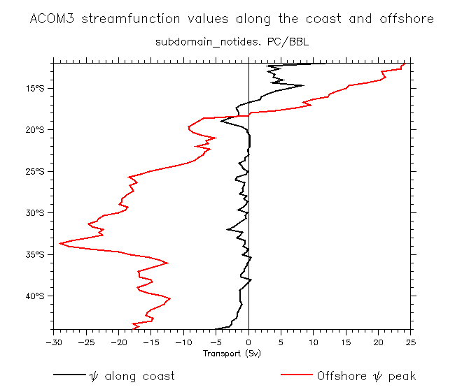
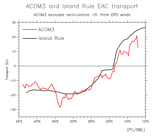
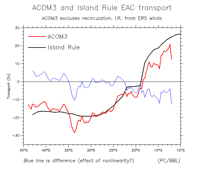
- EAC transport (difference in streamfunction across the WBC):
- Definition of EAC
- Values of Psi across the EAC
- ACOM3 and Island Rule transport (overlay difference)
- Regional winds
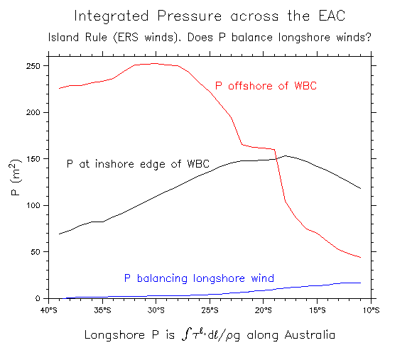
- Island Rule P across WBC (show P balancing longshore winds) (Misconceived)
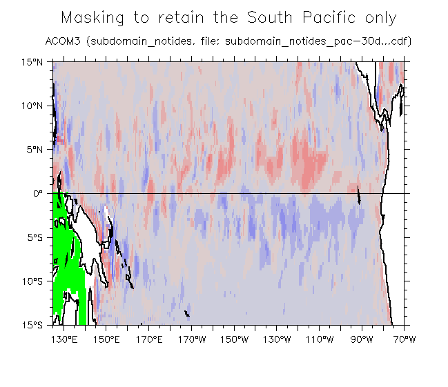
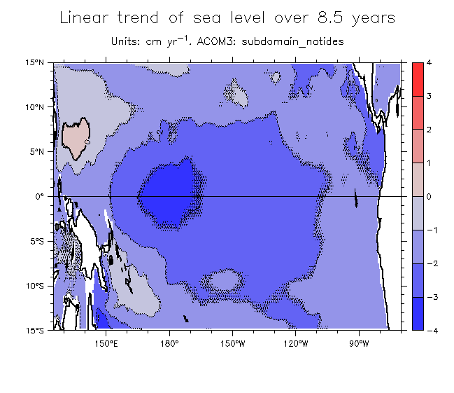
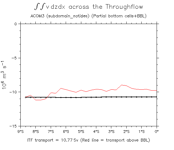
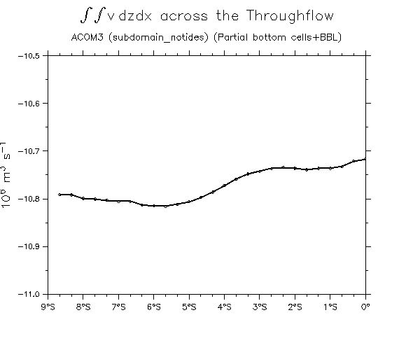
- What is the ACOM3 ITF/S.Pacific transport?
Confusion here. It is necessary to take into account the model's use of partial bottom cells and BBL ....
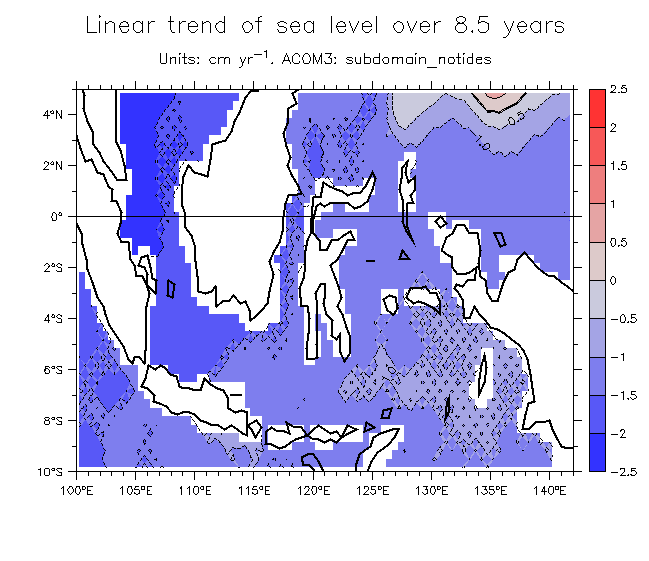
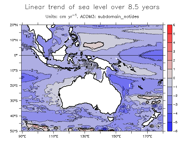
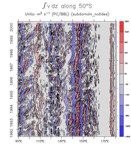
- S. Pacific boundaries S. Pacific transport Detail [Old one=no partial cells] Linear sea level trend
- ITF boundaries ITF transport Detail [Old one=no partial cells] Linear sea level trend (Entire subdomain region)
- Schematic of u and T points on the B-grid in a channel
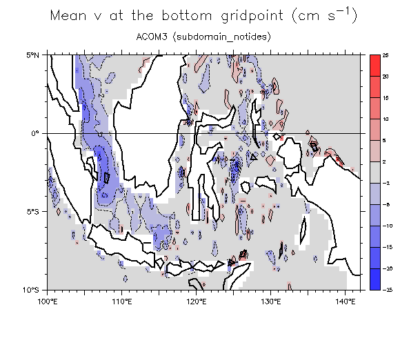
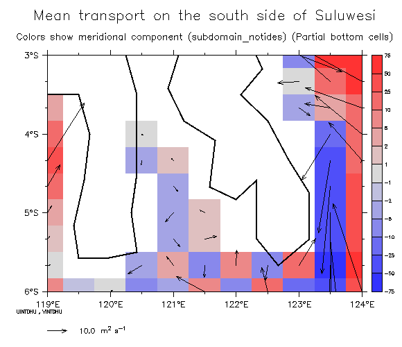
- Mean v at bottom gridpoints in the ITF Suluwesi transport
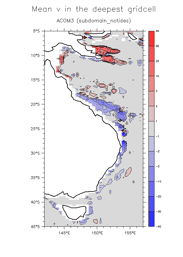
- Mean v at bottom gridpoints in the EAC Difference due to partial bottom cells: Depth Velocity
- BBL transport: Zonal Meridional
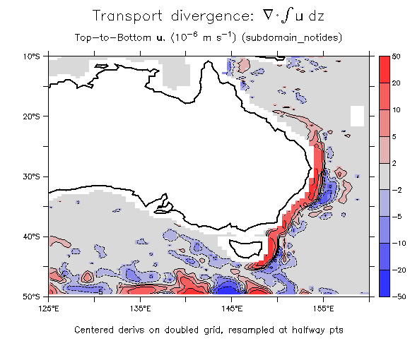
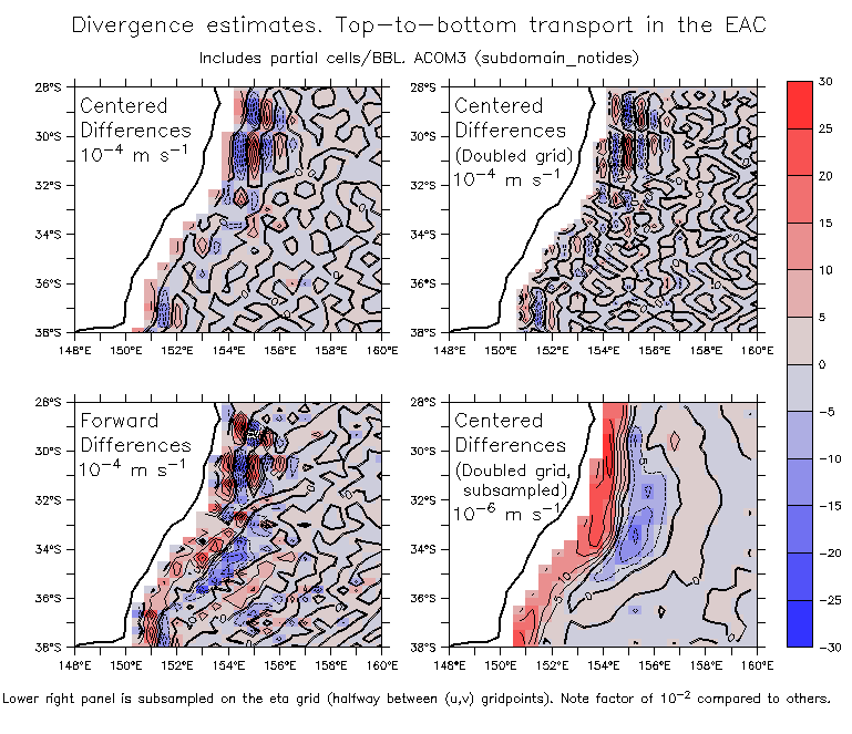
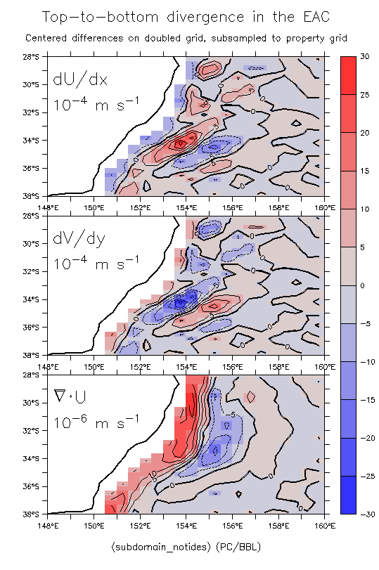
- Divergences: Subdomain region SE Australia
These divergences were found by (1) vertically integrating (u,v), including the partial bottom cells and BBL; (2) interpolating these transports onto a doubled grid; (3) taking centered differences; (4) subsampling to eta grid (centered between (u,v) cells). The values are very high! (1.e-6 m/s = 31.6 m/year)
Test streamfunction plots not blanking land: Entire region Detail 1 Detail 2
These are all the same streamfunction, but zooming in on the east coast of Australia (Note the effect of the non-zero divergence along 50°S causing some of the vertical stripes. Others are due to divergence along the Australian coast)
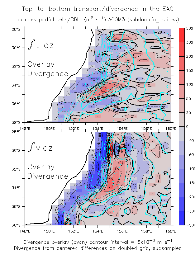
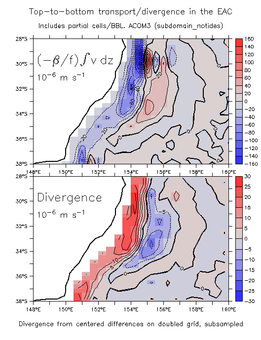
- Checking the divergences: u and v in the EAC Divergence estimates Overlay (Beta/f)v and Divergence du/dx and dv/dy (forward differences) du/dx and dv/dy (on doubled grid) Divergence and V (entire region) Zonal-average magnitude of divergence and V Time-dependent V along 50°S
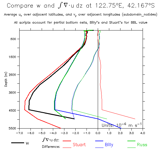
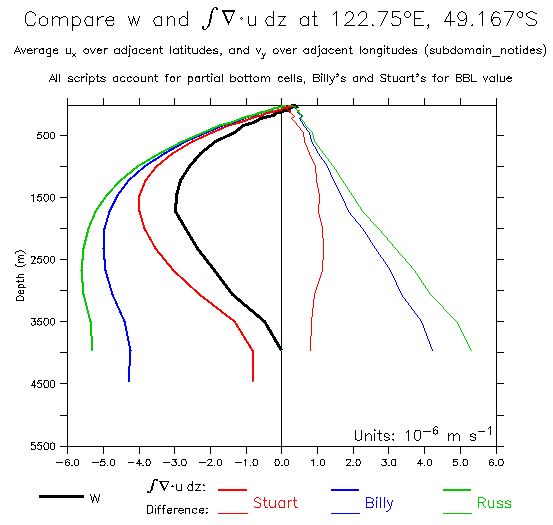
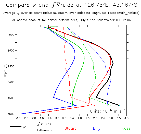
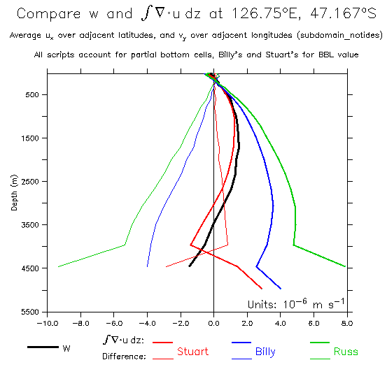
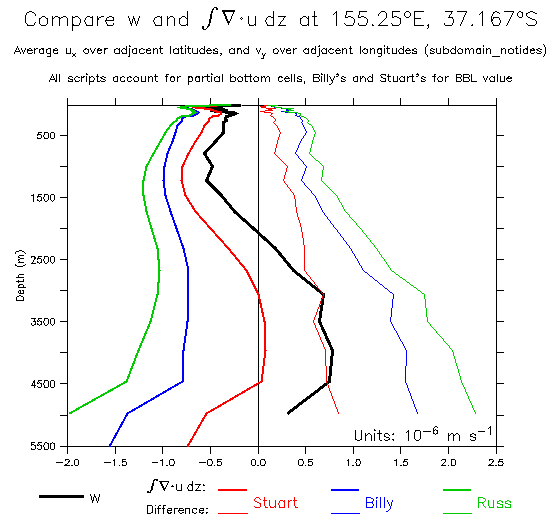
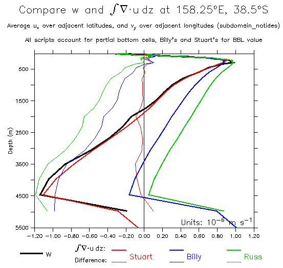
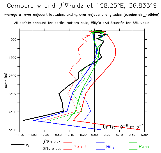
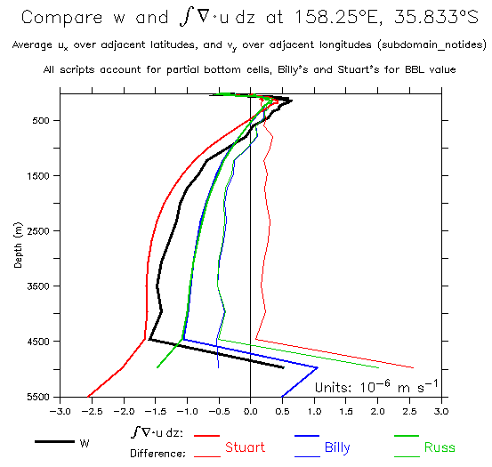
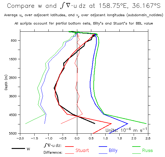
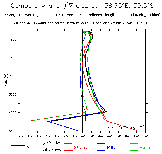
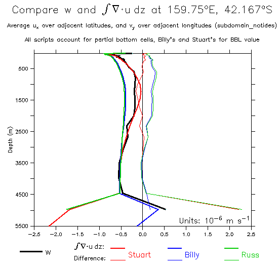
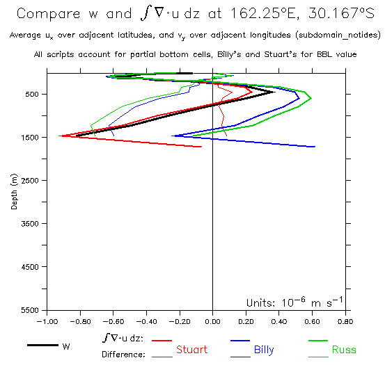
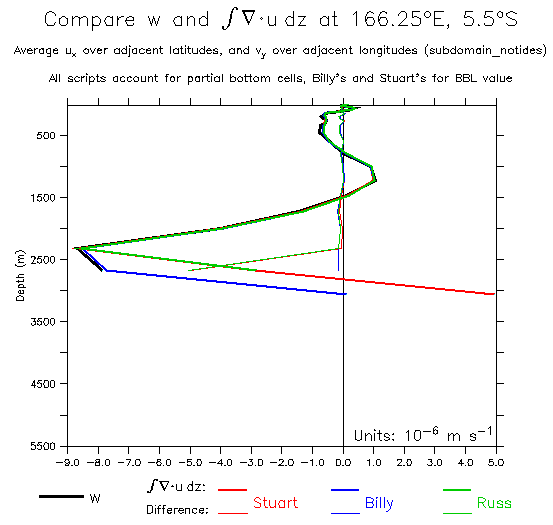
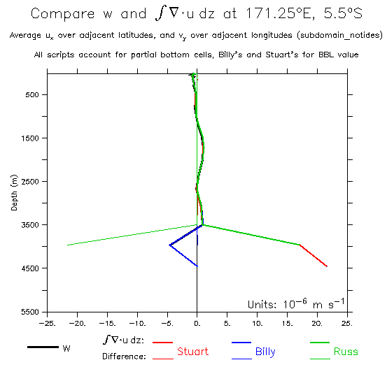
Compare w and integrated horizontal divergence:
- Line plots. These are a scattered selection of profiles showing w and the running downward integral of (u_x+v_y)dz. A restriction here is that only profiles where the derivatives could be calculated over 2 gridboxes in each direction all the way to the bottom were used (i.e. where the bottom is flat). Where there is a bottom slope all three scripts lose values at the bottom.
Stuart's and Russ's script makes no allowance for the partial bottom cells or BBL. Billy's script "correctly" finds the divergence from these (but the values are plotted here at the standard levels).
Note that at most of these locations, there is a large divergence signal in the partial bottom cell layer (with corresponding w signal). Also note that the contribution of BBL divergence (cyan line and dot at bottom of heavy blue line) is very close to what is needed to bring w (heavy black line) to zero at the bottom, showing that the BBL is essential to getting the divergence right.
The value of each line at the bottom of the profile measures the total divergence at each point (should be zero).
Note the different (automatic) scale in each plot.
123E,42S
123E,49S
127E,45S
127E,47S
155E,37.2S
155E,36.8S
155E,30S
158E,39S
158E,37S
158E,36S
159E,36S
159E,35S
160E,42S
162E,30S
166E,5S
171E,5S
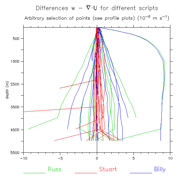
Differences: w - divergence for the above arbitrary selection of points
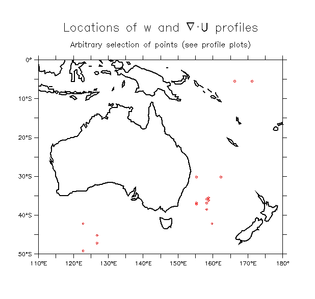
Map showing the above arbitrary selection of points
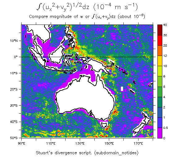
- Magnitude of the terms u_x and v_y, integrated to the partial bottom cell. This is about 100 times (not 10e4 times) the magnitude of the divergence (or of w).
- The three scripts: Stuart's Billy's Russ's
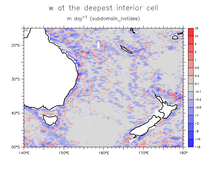
- w: w at the deepest interior cell v and (u,w) vectors at 33°S w at top and bottom cells at 33°S
Note to myself: many of these plots are not in the same directory as the html file.
Plots were made in /h/p/k/sverdrup/eac (Jul-Aug 02) and in /h/p/k/hobart (Jan 02 and Aug 02).
Plots sit in either /sverdrup or /sverdrup/islandrule
Related pages
Kessler home page
Figures page
EAC circulation work
Work done in Hobart
![[Old one=no partial cells]](../../sverdrup/merid-tran-across-pacific.gif)
![[Old one=no partial cells]](../../sverdrup/merid-tran-across-itf.gif)