Version 1.0 - Draft, 4/10/97

Copyright ©: 1995, 1996, 1997 George E. Mobus. All rights reserved.

The Adaptrode Learning Mechanism

George E. Mobus

Prior Affiliation: Western Washington University

Current Affiliation: University of Washington Tacoma, Institute of Technology

Abstract

A new neural learning rule is presented. This rule governs an adaptive mechanism that encodes auto- and cross-correlated signals across multiple time scales. As such it gives a better account of long-term memory phenomena than the traditional linear operator model from animal learning theory.

Neural Learning

Artificial neural networks (ANNs) are useful for solving a variety of problems in pattern recognition, classification and function approximation. An ANN's greatest benefit is in the fact that it learns how to solve the problem rather than being programmed. There are a number of neural learning rules in force today. These are generally classified into supervised (e.g., error backpropagation) and unsupervised (e.g., reinforcement) learning methods. In both cases, however, learning is accomplished by the modification of link or synaptic weights between neurons. Almost all learning rules involve modifications that ultimately lead to a stable weight matrix. Once the weights have stabalized the network has learned to recognize (or perform) whatever it will ever be asked to do. Such networks can be judged by how well they perform the target task.

Learning rules of the kind just described assume that the data set with which the networks are trained are statistically representative of the universe of data that the networks might ever see. For a large number of problem domains this may be a reasonable assumption. But for neural networks (or any machine learning system) to function in real-world environments they must be capable of on-going adaptation. Real environments are characterized as dynamic and indeterminate, having nonstationary statistical properties. Stated simply, things are constantly changing. Complicating this fact is that changes occur over many different scales of time and space. Thus some changes may be relevant to a particular problem but they are only local and/or temporary, relative to the range and life of the problem solver. Other changes may be gradual, global and permanent. In short, the problem solver cannot be said to make absolutely correct inferences about the current or future state of a problem domain since there is no such thing as an absolutely right answer.

Contact with Animal Learning - Real Neural Nets

If it is problematic to show a learning mechanism correct (say by convergence criteria) in natural environments then our recourse is to at least show that the mechanism's performance compares favorably with the de novo standard - learning in animals as evidenced by changes in behavior. When comparing mechanized learning with animal learning there are two major, interrelated concerns: Acquisition phenomena, including spatial and temporal relations; and memory phenomena. The former is the problem of what, when and how is learning accomplished. The latter is concerned with how (long) and under what conditions is a memory trace maintained. One might also include in this latter category, how memory traces are recalled and used.

Acquisition

What do animals learn? Since we are primarily interested in learning phenomena at the most basic level, we restrict this question to; what do very simple animals, with few synaptic links between stimulus and response, learn? Another, reasonable approach might be to ask: What do all animals learn? Or what is invariant in learning across all phylla?

One answer is that animals learn to associate cue stimuli from their environments with physiologically-important stimuli. Virtually all animals (complex enough to show learning ability) have sets of sensors that detect the presence of resources (such as the odor of food) or signal damage to the body. In most cases, these sensors are hard-wired to automatic or reflex responses such as orientation and flight. In addition, animals have sensors that have no a priori connection with such reflex responses. Sensory apparatus such as eye spots, chemodetectors, pressure detectors and the like provide additional data about the state of the environment but take on no necessary meaning with regard to the physiology of the creature. We call these free sensors, i.e., free of a priori semantic content.

However, since the environment is organized (no matter how chaotic) there will be some relationship between the state of the environment as detected by the free sensors and the occurrence of events which have physiological consequence. I conjecture that animal learning starts with the ability to learn those free sensory patterns (cues) that occur prior to the occurrence of physiologically-impacting events so as to use the former as predictors of the latter. Prediction can result in preemptive behavior that would tend to maximize benefit and/or minimize harm.

This kind of learning is precisely what is seen in conditioned learning such as Pavlovian or classical conditioning. Many considerations for what can be learned and when it is learned are taken up in this topic.

Memory

Animal learning theorists have, for some time, used a plausible model of memory called the linear operator model. In its basic form this is the exponential weighted moving average (EWMA) used to maintain a trace of a relevant state variable as a basis for forecasting a near-future state value. This model is used, for example, in foraging theory to explain how animals compute expectations of prey availability in recognized patches. It is also used to model the trace of short-term memory in conditioned learning theories. The reason this model is "plausible" is that it describes a "leaky integrator" which is a reasonable description of biophysical processes that must surely underlay memory. For short-term memory phenomena, EWMA-generated data points provide a good fit with empirical data. It is computationally efficient and under conditions where the statistics of the problem are effectively stationary, which is usually the case in short-term memory studies, EWMA can be shown to be mathematically equivalent to the windowed moving average. The linear operator model thus has provided a good working model for short-term memory phenomena.

However, the linear operator model does not do well when longer periods and long-term memory phenomena are evident in the behavioral data. For example, at the neurophysiological level, the EWMA does a reasonable job of modelling the excitatory post-synaptic potential (EPSP) of a short burst of action potential spikes. However, it cannot fit the data for intermediate- and long-term potentiation (LTP). At this point, most animal learning workers would and should feel uncomfortable with the idea that EWMA (describing a behavioral level phenomenon) should be used to describe a neuronal level phenomenon. It would be unreasonable to expect an abstract model like EWMA to account for cellular level events.

Adaptrode Learning

Nor should the EWMA model be expected to hold for all levels in the animal learning hierarchy. Nevertheless, whatever occurs at the cellular (indeed the subcellular) level accounts for key characteristics of what is seen at the behavioral level. This can best be seen if one restricts ones attention to the behavior of lower (i.e., more primitive) animal forms such as snails and planaria worms. Daniel Alkon [1] for example has developed a compelling model of the linkages between biophysical processes operating within individual neurons and the behavior of the marine nudibranch Hermissenda crassicornis. One of the more important aspects of Alkon's model is recognition of the various processes that operate over increasingly longer time scales. This model could provide a useful basis for multi-time scale memory traces as are seen in LTP studies. A summary of the correspondence between Alkon's model and the descriptions below is available.

Combining the usefulness of the EWMA (as a leaky integrator) and the multi-time scale model given by Alkon, I have developed a modified equation that behaves similarly to EWMA for strictly short-term memory but accommodates longer-term memory encoding as well. This model is called the adaptrode. A full description of the model appears in [2,3]. The model is summarized here.

Starting from the EWMA model, suppose that we want a response, r, from a linear operator at time t+1 based on its history and current stimulus. Thus:

where s is the stimulus signal and w is the memory trace ("weight").

The memory trace at time t+1 is given by:

where alpha lies between 0 and 1. Equation (2) is the EWMA. It can be seen in Fig. 1 that the trace of w falls off exponentially fast after the off-set of the stimulus. No longer-term memory trace is available beyond this limit. In the figure, two episodes of stimulus occur but the response of the operator to the second stimulus event is exactly that of the first event, as if the first had never happened.

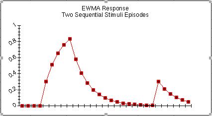
Figure 1.

A more likely situation would have the operator reacting more strongly to the second stimulus episode because the first had occurred and should not be treated as noise. In other words, we would like the operator response to retain a longer decay period reflecting a marginal memory of prior events. The adaptrode equation accomplishes this. Rearranging Eq. 1 to make this more explicit:

We now replace the last term in (3) with a new decay term and ad a shunting term to provide an upper bound:

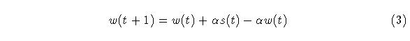
where delta is much less than alpha. The shunting expression in the second term is used to limit the size of w. In this model, the stimulus is either present or absent, 1 or 0. Figure 2 shows a comparison of the single level adaptrode with the EWMA model. As can be seen in the figure, the adaptrode behaves similarly to the EWMA but decays much more slowly. This means that the response to subsequent stimulus episodes will produce a slightly higher level. Delta is chosen so that a longer time window of decay can be achieved. Eventually, if no further episodes occur, the trace would decay back toward zero just as does the EWMA trace.

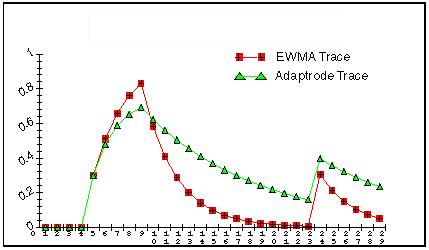
Figure 2.

Multi-time Scale Learning

While the use of a longer decay buys some additional memory it does not take into account patterns of stimulus episodes over longer time scales. Specifically, episodes may tend to cluster over intermediate scales, and, clusters themselves may cluster over even longer time frames. To address this problem a simple extension of the adaptrode equation is made. Let w_k denote a weight at level k and k lies between 0 and L, an index of the longest time scale. Then the computation of w_k at time t+1 is given by: $w_{k}(t+1) = w_{k}(t) + \alpha_{k} s<SUB>k</SUB>(t)(w_{k-1}(t) - w_{k}(t)) - \delta_{k} (w_{k+1}(t) - w_{k}(t))$

and

$w_{k-1} = 1, if k = 0 and w_{k-1} = 0 if k = L$

Note that a stimulus term, s_k(t), shows up in every level. This term will be used to implement associative learning in the next section.

This system of coupled difference equations are shown in [3] to produce a memory trace that provides longer term adaptations as seen in animal learning studies. Figure 3 shows a trace of a three level adaptrode. The top (red) trace is w₀, the middle (green) trace is w₁ and the bottom (blue) trace is w₂. s_1,2 were set to 1. Alpha and delta values for all levels have been chosen to exagerate the changes for viewing.

Figure 3.

As can be seen in Figure 3, the trace of w₁ rises more slowly than that of w₀ and, subsequently, the rise of w₂ is slower still. On the decay side, the trace of w₀ never falls below that of w₁ which, in turn, never falls below that of w₂. This "rising floor effect" is what provides a long-term memory trace. In the case shown in Figure 3, a single burst of input pulses results in a relatively small increase in the long-term trace. A subsequent input burst at some later time would cause w₀ to rise marginally faster and higher than it would have starting from zero. However, if over a longer time period, a number of burst episodes are experienced, the value ofw₂ (and, due to the floor, w₁ and w₀) would be much higher. Thus the impact of subsequent bursts on the rise of w₀ and, consequently, the output response of the adaptrode, would be much higher. This constitutes a "strong" long-term memory trace. On the other hand, if over the longer period, no (or few) episodes are experienced, then all of the traces will decay (albeit asymptotically) back to the ground state thus elliminating the trace. The adaptrode provides an "activity-dependent" memory mechanism. That is, it encodes short, intermediate and long-term traces that are proportional to activity of the input. This model corresponds qualitatively with a variety of neurophysiological models such as nonassociative long-term potentiation and habituation.

Associative Learning

Thus far the adaptrode model has addressed single channel or nonassociative, activity-dependent stimulus memory. There are a number of nonassociative memory phenomena such as habituation and sensitization for which this model might serve. Associative learning is, however, the more dominant, and arguably the more important, form of interest to us. Associative learning occurs when a correlation between two (or more) stimulus signals exists. The often referenced Hebb rule is of this sort [4]. A stronger form of association is found in what I have called causal correlations[2,3](see also [5] for a discussion of the historical context of this). In such an association an episode of one of the two stimulus types must routinely precede an episode of the second type by some small time lag. Where a "strong" correlation exists between two such signals then the occurrence of an episode of the first type signal can be used as a predictor of an episode of the second type.

An adaptrode network can be used to implement a correlation encoding mechanism. Consider two signals, denoted s_{0, c} and s_{0, u} (the index 0 represents the input to the zeroth level of the adaptrode; c stands for conditionable and u stands for unconditionable following conventions borrowed from animal learning theory) from two different but causally related environmental processes. Signal s_{0, u} is taken as having mission-impacting (e.g., physiological) consequences while s_{0, c} is detected by a free sensor as described above. Let r_c be the response of the adaptrode receiving the s_{0, c} signal and r_u be the reponse of the adaptrode receiving the s_{0, u} signal according to a set of equations based on (5) with appropriate settings for all parameters. Now let s_1,c(t) = G[r_u(t),r_c(t)], be a function. That is, the response of the adaptrode recieving the consequential input signal will be used as the input to the first level of the adaptrode receiving the non-consequential input as shown here in Figure 4.

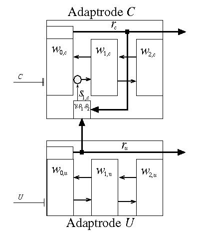
Figure 4.

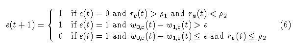
Now the function G[] will be given in two stages for clarity. We do this by defining an enabling switch, e(t) which is on (1) or off (0), depending on a specific temporal relationship between the onset of responses r_c and r_u. Specifically:

The constants, rho₁ and rho₂ are chosen so that r_c must have been on the rise and achieved some minimal value before r_u starts to rise in order to enable the function. The second condition in (6) assures that the function will remain enabled (once it has been enabled by the first condition) until the value of w_0,c has decayed down to near that of w_1,c by a small (<< 1) epsilon. The function is disabled when the last condition is met, and remains disabled until the first condition is met again. What this means is that if onset of the unconditionable stimulus, s_0,u, occurs prior to the onset of the conditionable stimulus, s_{0, c}, then the function, G[] remains disabled and s_1,c stays at zero (see Equation (7) below). This "latching" function is what establishes the unidirectional temporal ordering required by causal conditioning encoding. The time lag between the onset of signals (the opening of the window of opportunity) is controlled by the selection of rho_1,2.

The second stage of G[] is given by equation (7):

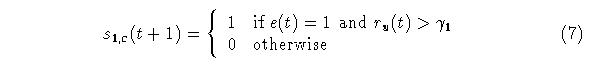
The function of gamma in (7) is to control the timing of the peak of correlation and, in combination with the decay rate of w₀,c the closing of the window of opportunity.

Equations (6) and (7) introduce additional parameters into the model. However, values of rho₁, rho₂, epsilon and gamma can be estimated from empirical data regarding the peak of association in classical conditioning experiments [3]. Additionally, by setting rho₁ = 0 and rho₂ = 1, it is possible to encode noncausal associations, i.e., standard correlations, in the A_c adaptrode. By making A_c and A_u reciprocal it is possible to encode standard cross-correlations which is applicable to traditional spatial pattern learning.

Figure 5 shows a graph of the three-level adaptrode when the G[] function is in force. In this graph the onset of the r_u response comes a sufficient number of time steps after the onset of r_c, as evidenced by the rise of w₀, so that the function is enabled. The final equilibrium value of w₁ is thus determined by how much time lags between the offset of s_0,c and the onset of s_0,u. I have shown that this relationship results in this network producing the characteristic inverted "U" shaped acquisition curve found in conditioned learning [2,3].

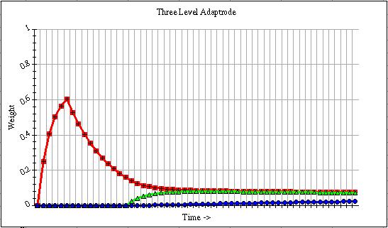
Figure 5.

Simulated Neural Networks

An artificial neuron or neuromime was developed using adaptrodes in place of traditional weights [3]. Simulations of a simple network of these neurons showed that some important long-term memory phenomena seen in the modification of behavior of animals but not currently explained by linear operator or other ANN models of conditioning were obtainable. Specifically in [2,3] I showed that it was possible to replicate memory savings after extinction and, indeed, after subsequent conditioning of the network on an orthogonal solution. The network was conditioned on one causal correlation solution (e.g. the presence of light meant reward) over an extended time scale. Evidence of the success of the conditioning was that the network responded to the cue signal alone by the output of a signal interpretable as "seek". Subsequently the cue stimulus was paired with the (semantically) opposite result (pain). The network demonstrated a short-term association formed with the newer condition by responding with an avoidance output. After several occurrences of the cue signal without subsequent reinforcement the short-term avoidance output extinguished. After extinction a mild seeking behavior reemerged showing that the network had retained a long-term memory of the longer time scale relationship between cue and reward. A small number of subsequent pairings of cue with reward brought the behavior back to its original level prior to the orthogonal treatment. These results may be interpreted as a solution to the problem of destructive interference experienced by other neural network learning models.

Conclusions

Learning and adaptation rules that operate in a single time domain cannot account for long-term behavioral modifications seen in animals. The adaptrode model presented here accommodates longer time scales and makes provision for an important class of associative learning, causal correlations. The latter is important because it allows animals to associate nonconsequential stimuli that may be causally related to the occurrence of stimuli having physiological (or mission impacting) consequences. The animal can use the occurrence of the former to predict the occurrence of the latter and take preemptive action to increase benefits or minimize harm.

The adaptrode model is also computationally efficient. Complexity is increased in terms of fixing a number of free parameters. However, experience gained in the course of conducting the above mentioned simulations suggest that these parameters are relatively easy to estimate from considerations of empirical studies in animal models. And from informal sensitivity studies I have conducted, it appears that most of the parameters are robust with respect to producing the desired behaviors.

Further explorations in using adaptrode-based neurons to build intelligent agents are underway. Both physical robots and their logical equivalents, knowbots situated in cyberspace, have been constructed and tested in limited, but nonstationary environments. Early results suggest that a behavior-based, bottom-up evolution of more complex intelligent agents is feasible.

References

Alkon, D., Memory Traces in the Brain, Cambridge University Press, 1987.
Mobus, G.E., Toward a theory of learning and representing causal inferences in neural networks , in Levine, D.S. and Aparicio, M (Eds.), Neural Networks for Knowledge Representation and Inference, Lawrence Erlbaum Associates, 1994.
Mobus, G.E., A multi-time scale learning mechanism for neuromimic processing, unpublished Ph.D. dissertation, University of North Texas, 1994.
Hebb, D.O., The Organization of Behavior, Wiley, New York, 1949.
Aparicio, M., Neural Computations for True Pavlovian Conditioning: Control of Horizontal Propagation by Conditioned and Unconditioned Reflexes, unpublished Ph.D. dissertation, University of South Florida, 1988.