Fluid flow of one or two fluids in pipes, annuli, and between flat plates.

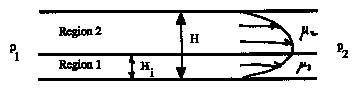
Figure 1. Flow of two immiscible fluids between flat plates

Consider the flow of two immiscible fluids between two flat plates in fully developed flow, as shown in Figure 1. One must solve for the location of the interface between the two fluids as well as for the velocity profile. If the flow is to be fully developed, then the pressure drop per length has to be the same in both fluids; otherwise there would be a transverse pressure gradient, which would lead to transverse flow, contrary to the fully developed assumption. For simplicity in this first example, take both fluids as Newtonian with a constant viscosity, which is different for the two fluids. The differential equations coming from the momentum balance are

The boundary conditions on the solid walls are that the velocity is zero.

There must also be compatibility conditions at the interface between the two fluids. We require that the velocity be continuous and that the shear stres be continuous (otherwise there would be generation of momentum at the interface).

This problem has an analytical solution (ref). Since the right-hand side of the differential equation is a constant, the velocity is a quadratic function of position in both regions, and the constants are adjusted to satisfy the differential equation (giving the constant in front of the x² term) and the boundary conditions. While the representation is messy, it is straightforward. Here we want to see how to solve the problem numerically, including more complicated cases in which the fluids are non-Newtonian (the viscosity then depends on shear rate), or the flow is in a pipe or annulus. Thus, we pose the following problems (sketched in Figure 2)

or

The boundary conditions are pipe flow are

The boundary conditions for annular flow are

The boundary conditions for flow between flat plates are

In this case, we ignore the term in the differential equation with (1/r), and think of r as x. We employ the finite difference method and the orthogonal collocation method on finite elements (in two regions) and compare them. More than two regions can be handled in a similar way. We note that color photographic film has many layers (20 or so), so this problem can be complicated but still realistic.

We also note that we don't need a numerical solution for two fluids with constant viscosities, but we can solve the problem numerically and compare with the exact solution. Once we have that numerical solution, though, it is relatively easy to solve for the non-Newtonian fluids, even though we could not do that analytically. Also, only minor variations were necessary to handle the pipe, annulus, or flat plates in the same code.

In some cases it is necessary to evaluate the differential equation at r = 0. Since both r and du/dr go to zero there, we employ l'Hopital's Rule

and the differential equation is