
Finite difference solution for flow of fluids in pipes, annuli, and between flat plates.
The problem is given elsewhere. The finite difference grid for this problem is shown in the figure.
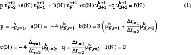
There are N1 points to the left of the interface and M points to the right, giving a total of N+M points. We use the finite difference form of the equation at all points interior to the fluid, two compatibility conditions at the N-th point, and a boundary condition at the first and last point. Due to the boundary conditions at the center of a pipe, for the pipe case we employ a false boundary (link) and write the differential equation at the first point, too, embedding the boundary condition there. The equations for points interior to the fluid are (following the format in BVP)
The compatibility condition for continuity of stress is
![]()
The velocity at point N is automatically continuous since we use only one variable for the velocity at point N. The boundary condition at the outer boundary gives
![]()
For the inner boundary, if we have an annulus or a solid flat plate the velocity is zero.
![]()
If we have a pipe or flat plate case using symmetry the derivative is zero.
![]()
We introduce a point, x0, beyond the first one (a false boundary) (link) and use a second order expression for the first derivative.
![]()
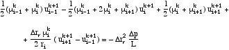
Thus, we use u2 = u0 in the second order expressions for the differential equation at r = 0. The governing equation at r = 0 is
We also use µ2 = µ0 ( the solution is symmetric about r = 0, i = 1_, and the equation becomes
Upon rearrangement, this is
![]()
These equations represent a set of nonlinear equations (if the viscosity depends on shear rate), or a set of linear equations if the viscosity is constant in each fluid region. For the nonlinear case, we employ version 3 outlined in the section on boundary value problems; the viscosity is evaluated using the shear rate at the last iteration, and then the velocity at all points is solved for simultaneously. Since the viscosity might be wrong (it was evaluated using a possibly incorrect shear rate), the viscosity is updated and the iteration continued to convergence.
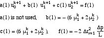
The form of the finite difference equations at the point i is

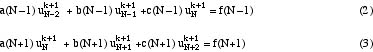
where the terms a(i), b(i), and c(i) are evaluated using the viscosity at the previous iteration. Since there are only three unknowns, the matrix problem is a tri-diagonal system of equations, which should be solved using special methods. The equations representing the boundary conditions are special. For the annulus and flat solid plate the boundary condition at the first point is
![]()
For the pipe and flat plate with symmetry, the condition at the first point is the transformed equation.
For the last point, all geometries, the boundary condition is
![]()
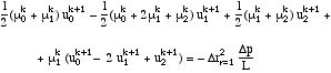
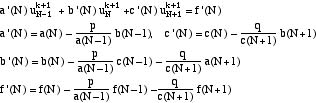
For the compatibility condition at point N, we have the condition
![]()
This equation is written in the form
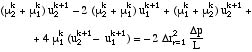
This condition violates the tri-diagonal nature of the matrix equations. If the problem is small, then we can just put the equations into one big matrix, even though most of the element entries are zero. It is more efficient, though, to employ the features of the tri-diagonal matrix. To do that, we have to transform the last equation to make it tridiagonal. We have an equation on each side of the interface:
Thus, we multiply the Eq. (2) by a factor and add it to Eq. (1) in such a way that the first term drops out. The factor is p / a(N1). We do the same thing with the third equation; the factor is q / c(N+1). Now the compatibility equation is
Now the entire problem is tridiagonal and can be quickly solved using this code. To verify the accuracy of the code, consider the flow rate in region 2 as the mesh is refined.
Flow rate in region 2 when the interface is half way between two flat plates.
| Number of grid points per region | Flow rate in region 2 |
|---|---|
| 3 | 132.155 |
| 6 | 133.891 |
| 12 | 134.325 |
| 24 | 134.434 |
The values are and they show the expected second order convergence with mesh size (link). Even with 7 total points, the flow rate is accurate within a few per cent. However, the exact solution is only a quadratic function of position in the two regions, and the finite difference method should give the exact solution for flow rate in that case. When the trapezoid rule for quadrature is replaced by Simpson's Rule the flow rates are exact, as expected. Thus, the errors in the table are due entirely to the quadrature method used, in this case.
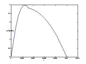
When the problem is solved using the parameters given in the code, the results are plotted in the figure.

Because the viscosity in region 1 is much smaller than that in region 2, there is more flow in region 1, leading to the bulge. When the interface is only 30% of the way across, the solution is shown in the next figure.
Next consider the case of a non-Newtonian fluid. Now the viscosity must be evaluated at each grid point using a subfunction. Here a made-up problem uses the formula for viscosity
![]()
Convergence of the iterations is very fast, with only xxx iterations needed. The grid refinement also shows that the numerical problem has converged to the solution of the differential equation. Note that the velocity profile is flatter over part of the region for the non-Newtonian case.
We note that we didn't need a numerical solution for two fluids with constant viscosities, but we could solve the problem numerically and compare with the exact solution. Once we had that numerical solution, though, it was relatively easy to solve for the non-Newtonian fluids, even though we could not do that analytically. Also, only minor variations were necessary to handle the pipe, annulus, or flat plates. If one used the same function for viscosity in both regions, one would get the solution for a single fluid. The only difference between this code and one for only one phase is that this code uses a compatibility condition at the N-th point, whereas a code for one phase would use the differential equation there. By running the code with µ1 = µ2, you can see that this makes little difference.