Application of Orthogonal Collocation

Let us apply the orthogonal collocation method to the nonlinear heat transfer problem (link).

The collocation points are shown in the figure. There are N interior points plus one at each end. and the domain is always transformed to lie on 0 to 1.

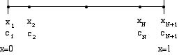
Figure: Orthogonal Collocation Points

The orthogonal collocation method is applied by requiring the trial solution to satisfy the boundary conditions, which are at collocation points x₁ and x_N+2.

⁽¹⁾

Then the residual is set to zero at the interior collocation points.

In the orthogonal collocation method, this is written as

⁽²⁾

We use Table I to obtain the matrices representing the first and second derivatives. Equations (1) and (2) represent N+2 equations for the N+2 unknowns {y_j}.

In the first approximation, N = 1, N+2 = 3, we have three collocation points.

The collocation equation (2) is then

If the matrices are applied from Table I we get

When the boundary conditions (1) are applied we get

Solving this equation for y₂ gives y₂ = 0.579156.

The flux at x = 0 is given by

When the orthogonal collocation matrices are inserted from Table I we get

Using the solution gives the flux as 1.3166. The flux at x = 1 is given by

When the orthogonal collocation matrices are inserted from Table I we get

Using the solution gives the flux as 1.3667. There is only a 4% difference in these fluxes, which might suggest that the answer is pretty good. The higher approximations show, however, that the error (compared with the exact solution and higher approximations) is 10%.

When four collocation points are used (N+2=4), or two interior points, the values for fluxes at either side are 1.4881 and 1.4926, which are within 0.2% of each other and are within 0.67% of the exact solution. The error in the flux decreases as the number of terms is increased, as illustrated in Figure 1.

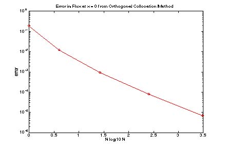
Figure 1. Error in Flux at x = 0

The solutions are plotted in Figure 2, and they are hardly distinguishable from the exact solution.

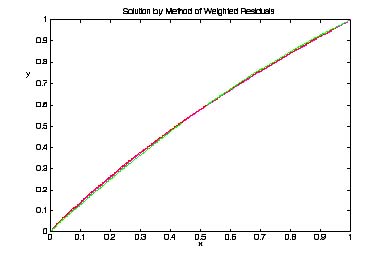
Figure 2. OC Solution, N = 1 and 2 (green), and exact solution (red)

The residual can be evaluated once the solution is known, too. It should be zero at the collocation points, and we hope it gets smaller as the number of terms increases. Figures 3-5 show that this is true.

Figure 3. Residual for N = 1 and N = 2.

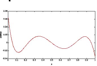
Figure 4. Residual for N = 5.

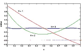
Figure 5. Residual for N = 1, 2 and 5.

Take Home Message: Orthogonal Collocation needs only a few terms to solve many problems very accurately.