You are welcome (and encouraged) to work with others, but each individual must submit their own writeup.
You are welcome to use your preferred computational toolkit – upload the commented sourcecode alongside your writeup (e.g. the .ipynb file).
You are welcome to consult research articles and other materials – upload a .pdf of the article alongside your writeup and indicate which references were used where in the writeup.
linear quadratic regulation (16 pts)
Consider the discrete-time linear quadratic regulator problem (DT-LQR)
where \(P_t\), \(\{Q_s\}_{s=\tau}^{t-1}\), \(\{R_s\}_{s=\tau}^{t-1}\) are given symmetric positive-definite matrices.
In this problem, you’ll apply Bellman’s dynamic programming principle to determine the optimal control, then verify this control is the same one obtained by a descent algorithm.
Determine the optimal control and value at time \(\tau = t\) (i.e. minimize \(c_t\) with respect to \(u_t\), and let \(v^*_t = c_t(x^*,u^*)\) denote the optimal value that can be obtained at time \(t\)).
The problem description can be written in math form as: \[\min_{u_t} c_{\tau=t}(x,u) = \frac{1}{2} x_t^\top P_t x_t + \frac{1}{2}\sum_{s=\tau=t}^{t-1} x_s^\top Q_s x_s + u_s^\top R_s u_s \]\[\min_{u_t} c_{t}(x,u) = \frac{1}{2} x_t^\top P_t x_t\] Since by definition (and a change of variable), \[x_{t} = A_{t-1} x_{t-1} + B_{t-1}u_{t-1}\] Substituting \(x_t\) in \(c_t(x,u)\), we can conclude that equation \(c_t(x,u) = \frac{1}{2} x_t^T P_t x_t\) is independent of \(u_t\), thus any input is optimal. For simplicity, I will choose \(u_t^* = 0\). The optimal value is \[v_t^* = c_t = \frac{1}{2} x_t^T P_t x_t\]
Determine the optimal control and value at time \(\tau = t-1\) (i.e. minimize \(c_{t-1}\) with respect to \(u_{t-1}\), and let \(v^*_{t-1} = c_{t-1}(x^*,u^*)\) denote the optimal value that can be obtained at time \(t-1\)).
First, let’s put \(c_{t-1}\) in math form \[c_{\tau=t-1}(x,u) = \frac{1}{2} x_t^\top P_t x_t + \frac{1}{2}\sum_{s=\tau=t-1}^{t-1} x_s^\top Q_s x_s + u_s^\top R_s u_s \]\[c_{t-1}(x,u) = \frac{1}{2} x_t^\top P_t x_t +\frac{1}{2} x_{t-1}^\top Q_{t-1} x_{t-1} +\frac{1}{2} u_{t-1}^\top R_{t-1} u_{t-1}\] Substituting \(x_t = A_{t-1} x_{t-1} + B_{t-1} u_{t-1}\) and differentiating \(c_{t-1}\) with respect to \(u_{t-1}\), we find \[ D_{u_{t-1}} c_{t-1} = (A_{t-1} x_{t-1} + B_{t-1} u_{t-1})^T P_t B_{t-1}+u_{t-1}^T R_{t-1} \] Solving \(D_{u_{t-1}} c_{t-1} = 0\) for \(u_{t-1}^*\) yields \[ u_{t-1}^* = -(B_{t-1}^T P_t B_{t-1} + R_{t-1})^{-1} B_{t-1}^T P_t A_{t-1} x_{t-1}. \] Notice that \(D_{u_{t-1}}^2 c_{t-1} = R_{t-1} + B_{t-1}^T P_t B_{t-1}\), which is a symmetric positive-definite matrix, so the input we computed is a strict local minimizer. With that said, we’ll derive a simplified expression for the optimal value in the next step.
Note that the optimal control is linear in state and the optimal value is quadratic in state (i.e. determine \(K_{t-1}\) and \(P_{t-1}\) such that \(u_{t-1} = K_{t-1} x_{t-1}\) and \(v^*_{t-1} = c_{t-1}(x^*,u^*) = x_{t-1}^T P_{t-1} x_{t-1}\)).
Use the substitution in (c.) to generalize the calculation in (b.) to derive a recursive formula to compute the optimal control and value at any time \(s\in [\tau,t]\).
We can prove by induction that suppose \[ K_s = (B_{s}^T P_{s+1} B_{s} + R_{s})^{-1} B_{s}^T P_{s+1} A_{s} \]\[ P_s = (A_{s} - B_{s} K_{s})^T P_{s+1} (A_{s} - B_{s} K_{s}) + Q_{s} + K_{s}^T R_{s} K_{s}\] , then the optimal input and optimal value at any time \(s\) are respectively \[ u_s^* = -K_s x_s\]\[ v_s^* = \frac{1}{2} x_s^T P_s x_s\] This means that if we assume \(A\), \(B\), \(Q\), \(R\) and \(P_t\) are known from the system, we can recursively find \(K_s\) and \(P_s\) in the reverse time order (i.e. \(s = t-1,t-2,...\)). $$$$ Note that the recursion for \(P_s\) is termed a Riccati difference equation; it is nonlinear, so not trivial to predict its asymptotic behavior as \(s\rightarrow-\infty\). It turns out that if \(A\), \(B\), \(Q\), and \(R\) are constant and \((A,B)\) is controllable, then the limit \(\lim_{s\rightarrow-\infty} P_s = P\) is well-defined and \(P\) satisfies the discrete algebraic Riccati equation\(A^T P A - (A^T P B)(R + B^T P B)^{-1}(B^T P A) + Q\).
Implement the recursion in (d.) numerically for the following system, which is a discretized linear spring-mass-damper (let \(\kappa,\beta,q,r,\Delta > 0\) be parameters that you can easily vary in your implementation):
import numpy as npfrom scipy import linalg as ladef riccati(A,B,Q,R,P):# optimal control is linear state feedback K_ = np.dot( la.inv(np.dot(B.T,np.dot(P,B)) + R), np.dot(B.T,np.dot(P,A)) )# optimal value is quadratic in state P_ = np.dot( (A - np.dot(B,K_)).T, np.dot(P, (A - np.dot(B,K_))) + Q + np.dot(K_.T, np.dot(R, K_)) )return K_,P_n =2m =1def lqr(t,kappa=1,beta=1,q=1,r=1,Delta=1e-1): A = np.identity(n) + Delta * np.array([[0,1],[-kappa,-beta]]) B = Delta * np.array([[0],[1]]) Q = q * np.identity(n) # running state cost R = r * np.identity(m) # running control cost K = np.zeros((t,m,n)) # linear state feedback gain matrix P = np.zeros((t+1,n,n)) # cost-to-go Pt = np.zeros((n,n)) # final state cost P[t] = Pt# loop over timesfor s inrange(t)[::-1]: # loop backward in time K[s],P[s] = riccati(A,B,Q,R,P[s+1])return A,B,Q,R,K,P
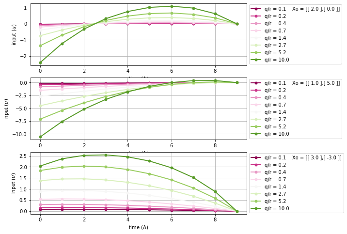
Investigate how the optimal controls vary with respect to the ratio \(q/r\) (i.e. let \(q/r\) range from \(0.1\) to \(10\), compute the optimal control input, describe the trend you observe, and provide a visualization that clearly illustrates this trend).
Code
from matplotlib import cmimport pylab as plt# plot variableslw =2# line widthms =10# markerfig = plt.figure(figsize=(8,8)); plt.clf()# a list of initial conditionsXo_list = [[[2],[0]],[[1],[5]],[[3],[-3]]] # TODO: can change here# system variablest =10# final timenum_q =8# number of q/r tests to considernum_e =len(Xo_list) # number of experiments# start experimentsfor exp inrange(num_e): u = np.zeros((t,m,1)) v = np.zeros((t)) x = np.zeros((t+1,n,1)) x[0] = Xo_list[exp] Xo_str =" Xo = [[ %0.1f ],"% x[0][0]+"[ %0.1f ]]"% x[0][1]for c,q inenumerate(np.logspace(-1,1,num=num_q)): A,B,Q,R,K,P = lqr(t,q=q,r=1.) # find all the system matricesfor s inrange(t): u[s] = np.dot(-K[s],x[s]) # calculate optimal input v[s] =0.5* np.dot( x[s].T, np.dot(P[s], x[s]) ) # calculate optimal value x[s+1] = np.dot(A,x[s]) + np.dot(B, u[s]) # calculate next state# illustrate optimal input over time plt.subplot(num_e,1,exp+1); plt.grid('on') plt.plot(u[:,0,0],'.-',lw=lw,ms=ms,color=cm.PiYG(1.*c/num_q),label="q/r = "+"%0.1f"% q+Xo_str) plt.ylabel(r'input ($u$)') plt.legend(loc="center left", bbox_to_anchor=(1,0.5)) plt.xlabel(r'time ($\Delta$)') Xo_str =""
/usr/local/lib/python3.6/dist-packages/ipykernel_launcher.py:37: MatplotlibDeprecationWarning: Adding an axes using the same arguments as a previous axes currently reuses the earlier instance. In a future version, a new instance will always be created and returned. Meanwhile, this warning can be suppressed, and the future behavior ensured, by passing a unique label to each axes instance.
From the plots, we notice when state error \(q\) is much more costly than input effort \(r\) (green curves), optimal inputs tend to have greater magnitude so the state error decreases faster. Contrarily, when \(q/r\) is small (pink curves), small inputs are applied and state error decreases slowly.
Verify your implementation in (e.) by applying a descent algorithm to approximate the optimal input on time horizon \(t = 10\cdot\Delta\) and \(t = 100\cdot\Delta\) for the following initial conditions with \(\kappa,\beta,q,r = 1\), \(\Delta = 0.1\):
\[x_1 = (1,0),\ x_2 = (0,1).\]
Hint: you can directly apply simple random search, or use finite differences to approximate the gradient. To apply steepest descent or Newton-Raphson, you’ll need to analytically differentiate the cost with respect to the control input applied at each timestep.
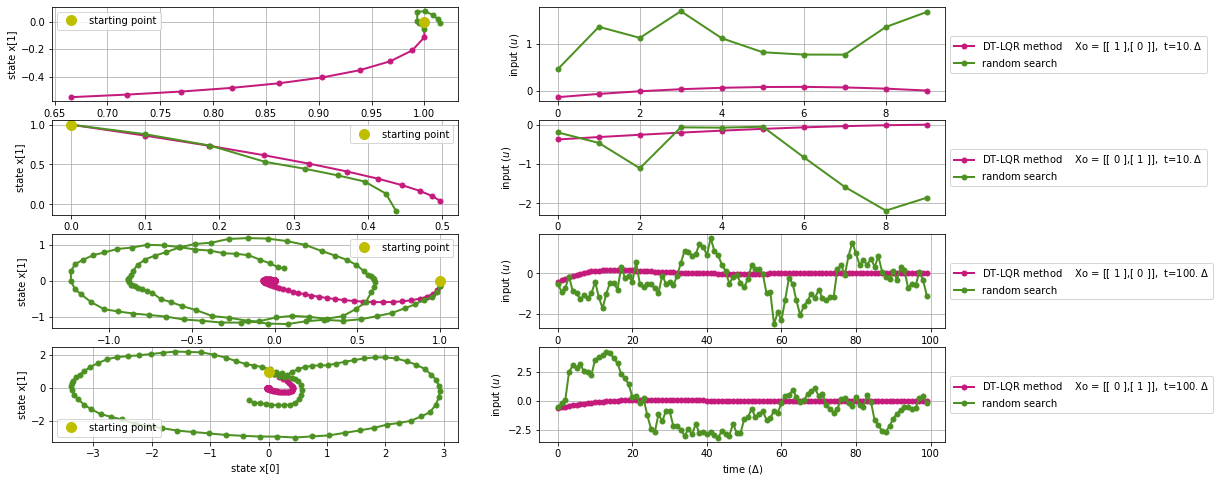
First, lets use the DT-LQR approach to determine a series of optimal inputs (pink curves). Then, we can try calculating the optimal inputs using random search algorithm (green curves). Finally, we illustratively compare the results by showing both the state trajectory and input over time plot. We can notice that although the input sequence dont necessarily look similar, the overall state x seem to spiral inward toward (0,0) which is a good sign. Also, the Dt-LQR method drives input to approach 0 as time moves alongs.
Code
from matplotlib import cmimport pylab as pltfrom scipy.misc import derivativeimport random# plot variableslw =2# line widthms =10# markerfig = plt.figure(figsize=(16,8)); plt.clf()# a list of initial conditionsXo_list = [[[1],[0]],[[0],[1]]] # system variablesDelta =0.1# time stept_list = [10,100] # final timenum_e =len(Xo_list) # number of experimentscnt =0# a counter that keeps track of iterations# cost functiondef c(w,xo,t): x = np.zeros((t+1,n,1)) x[0] = xo c =0.for s inrange(t): c +=0.5* np.dot(x[s].T, np.dot(Q, x[s])) + np.dot(w[s].T, np.dot(R, w[s])) x[s+1] = np.dot(A,x[s]) + np.dot(B,w[s]) return c,xdef random_search(u,s,t,xo): step =0.1 u_tmp = u v_best =float('inf')for i inrange(100): u_tmp[s] = u[s]+random.uniform(-step,step) v_tmp, x_tmp = c(u_tmp[:s],xo,s)if v_tmp < v_best: u_best = u_tmp # calculate optimal input v_best = v_tmp # calculate optimal value x_best = x_tmp # calculate next statereturn u_best, v_best, x_best# start experimentsfor t in t_list:for exp inrange(num_e):## ======================== DT-LQR method ======================== u = np.zeros((t,m,1)) v = np.zeros((t)) x = np.zeros((t+1,n,1)) cnt = cnt +1 x[0] = Xo_list[exp] Xo_str =" Xo = [[ %0.f ],"% x[0][0]+"[ %0.f ]]"% x[0][1] A,B,Q,R,K,P = lqr(t,Delta=Delta) # find all the system matricesfor s inrange(t): u[s] = np.dot(-K[s],x[s]) # calculate optimal input v[s] =0.5* np.dot( x[s].T, np.dot(P[s], x[s]) ) # calculate optimal value x[s+1] = np.dot(A,x[s]) + np.dot(B, u[s]) # calculate next state# illustrate optimal input over time plt.subplot(len(t_list)*num_e,2,2*cnt); plt.grid('on') plt.plot(u[:,0,0],'.-',lw=lw,ms=ms,color=cm.PiYG(0.1),label="DT-LQR method"+Xo_str+", t=%0.f$.\Delta$"%t) plt.ylabel(r'input ($u$)') plt.legend(loc="center left", bbox_to_anchor=(1,0.5)) plt.xlabel(r'time ($\Delta$)') plt.subplot(len(t_list)*num_e,2,2*cnt-1); plt.grid('on') plt.plot(x[:,0,0],x[:,1,0],'.-',lw=lw,ms=ms,color=cm.PiYG(0.1)) plt.ylabel(r'state x[1]') plt.xlabel(r'state x[0]')## ===================== random search method ===================== u_prev = u[0] u = np.zeros((t,m,1)) v = np.zeros((t)) x = np.zeros((t+1,n,1)) x[0] = Xo_list[exp] u[0] = u_prevfor s inrange(t): v[s] =float('Inf')if s >0: u[s] = u[s-1] u, v[s], x[:s+1,:,:] = random_search(u,s,t,x[0])# illustrate optimal input over time plt.subplot(len(t_list)*num_e,2,2*cnt); plt.grid('on') plt.plot(u[:,0,0],'.-',lw=lw,ms=ms,color=cm.PiYG(0.9),label="random search") plt.ylabel(r'input ($u$)') plt.legend(loc="center left", bbox_to_anchor=(1,0.5)) plt.xlabel(r'time ($\Delta$)') plt.subplot(len(t_list)*num_e,2,2*cnt-1); plt.grid('on') plt.plot(x[:t-1,0,0],x[:t-1,1,0],'.-',lw=lw,ms=ms,color=cm.PiYG(0.9)) plt.plot(x[0,0,0],x[0,1,0],'o',lw=lw,ms=ms,color='y',label="starting point") plt.legend(loc="best") plt.ylabel(r'state x[1]') plt.xlabel(r'state x[0]')
/usr/local/lib/python3.6/dist-packages/ipykernel_launcher.py:86: MatplotlibDeprecationWarning: Adding an axes using the same arguments as a previous axes currently reuses the earlier instance.  In a future version, a new instance will always be created and returned.  Meanwhile, this warning can be suppressed, and the future behavior ensured, by passing a unique label to each axes instance.
/usr/local/lib/python3.6/dist-packages/ipykernel_launcher.py:91: MatplotlibDeprecationWarning: Adding an axes using the same arguments as a previous axes currently reuses the earlier instance.  In a future version, a new instance will always be created and returned.  Meanwhile, this warning can be suppressed, and the future behavior ensured, by passing a unique label to each axes instance.
Bonus: analytically differentiate the cost with respect to the control input applied at each timestep one or two times to implement steepest descent or Newton-Raphson algorithms to approximate the optimal control.
Now consider the infinite time-horizon problem with time-invariant dynamics:
\[\min_u c(x,u) \ \text{s.t.} \ x_{s+1} = A x_s + B u_s,\]\[c(x,u) = \frac{1}{2}\sum_{s=0}^{\infty} x_s^\top Q x_s + u_s^\top R u_s,\]
where \(A\), \(B\), \(Q\), and \(R\) do not vary in time. Noting that the system from (e.) is time-invariant, solve the LQR problem on an “infinite” time horizon: iterate the recursion from (d.) many times and plot the entries of the \(P\) matrix versus iteration number. Compare with the result obtained from solving the discrete algebraic Riccati equation
\[ X = (A - B K)^\top X (A - B K) + K^\top R K + Q,\ K = (B^\top X B + R)^{-1} B^\top X A \]
using the solve_discrete_are routine from the scipy.linalg module or the dare routine from the python-control module (execute !pip install python-control in Colab to make this module available).
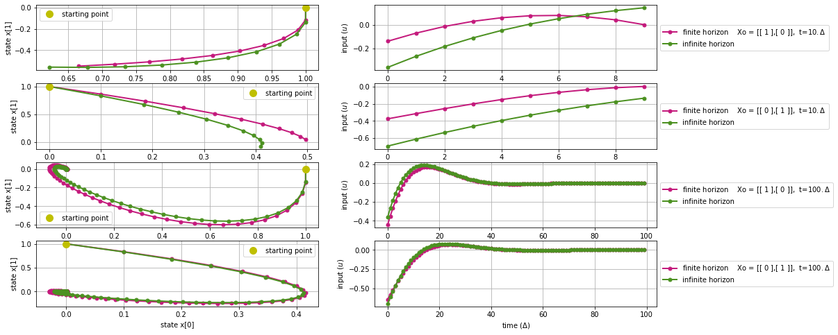
In this problem, we compare the DT-LQR solutions from the finite horizon and infinite horizon case. First, lets use the DT-LQR approach which is the same as the approach we used in problem (g) to determine a series of optimal inputs (pink curves). Then, we can try calculating the optimal inputs using infinite time horison solve_discrete_are routine (green curves). Finally, we illustratively compare the results. As one may notice, as the number of iterations increases, the control input sequence from the finite horizon case gets closer to the infinite time horison solution.
Code
from matplotlib import cmimport pylab as pltfrom scipy.misc import derivativeimport random# plot variableslw =2# line widthms =10# markerfig = plt.figure(figsize=(16,8)); plt.clf()# a list of initial conditionsXo_list = [[[1],[0]],[[0],[1]]] # system variablesDelta =0.1# time stept_list = [10,100] # final timenum_e =len(Xo_list) # number of experimentscnt =0# a counter that keeps track of iterationsdef discete_are(A,B,Q,R):"""Solve the infinite time horizon discrete time lqr controller. x[k+1] = A x[k] + B u[k] cost = sum x[k].T*Q*x[k] + u[k].T*R*u[k] """# Riccati Recursion: the min-cost-to-go matrix # Try to solve the ricatti equation, Bertsekas, p.151 X = np.matrix(scipy.linalg.solve_discrete_are(A, B, Q, R))#compute the LQR gain K_are = np.matrix(scipy.linalg.inv(B.T*X*B+R)*(B.T*X*A)) return K_are# start experimentsfor t in t_list:for exp inrange(num_e):## ======================== finite horizon ======================== u = np.zeros((t,m,1)) v = np.zeros((t)) x = np.zeros((t+1,n,1)) cnt = cnt +1 x[0] = Xo_list[exp] Xo_str =" Xo = [[ %0.f ],"% x[0][0]+"[ %0.f ]]"% x[0][1] A,B,Q,R,K,P = lqr(t,Delta=Delta) # find all the system matricesfor s inrange(t): u[s] = np.dot(-K[s],x[s]) # calculate optimal input v[s] =0.5* np.dot( x[s].T, np.dot(P[s], x[s]) ) # calculate optimal value x[s+1] = np.dot(A,x[s]) + np.dot(B, u[s]) # calculate next state# illustrate optimal input over time plt.subplot(len(t_list)*num_e,2,2*cnt); plt.grid('on') plt.plot(u[:,0,0],'.-',lw=lw,ms=ms,color=cm.PiYG(0.1),label="finite horizon"+Xo_str+", t=%0.f$.\Delta$"%t) plt.ylabel(r'input ($u$)') plt.legend(loc="center left", bbox_to_anchor=(1,0.5)) plt.xlabel(r'time ($\Delta$)') plt.subplot(len(t_list)*num_e,2,2*cnt-1); plt.grid('on') plt.plot(x[:,0,0],x[:,1,0],'.-',lw=lw,ms=ms,color=cm.PiYG(0.1)) plt.ylabel(r'state x[1]') plt.xlabel(r'state x[0]')## ===================== infinite horizon ===================== u = np.zeros((t,m,1)) v = np.zeros((t)) x = np.zeros((t+1,n,1)) x[0] = Xo_list[exp] K_are = discete_are(A,B,Q,R)for s inrange(t): u[s] = np.dot(-K_are,x[s]) # calculate input x[s+1] = np.dot(A,x[s]) + np.dot(B, u[s]) # calculate next state# illustrate optimal input over time plt.subplot(len(t_list)*num_e,2,2*cnt); plt.grid('on') plt.plot(u[:,0,0],'.-',lw=lw,ms=ms,color=cm.PiYG(0.9),label="infinite horizon") plt.ylabel(r'input ($u$)') plt.legend(loc="center left", bbox_to_anchor=(1,0.5)) plt.xlabel(r'time ($\Delta$)') plt.subplot(len(t_list)*num_e,2,2*cnt-1); plt.grid('on') plt.plot(x[:,0,0],x[:,1,0],'.-',lw=lw,ms=ms,color=cm.PiYG(0.9)) plt.plot(x[0,0,0],x[0,1,0],'o',lw=lw,ms=ms,color='y',label="starting point") plt.legend(loc="best") plt.ylabel(r'state x[1]') plt.xlabel(r'state x[0]')
/usr/local/lib/python3.6/dist-packages/ipykernel_launcher.py:73: MatplotlibDeprecationWarning: Adding an axes using the same arguments as a previous axes currently reuses the earlier instance.  In a future version, a new instance will always be created and returned.  Meanwhile, this warning can be suppressed, and the future behavior ensured, by passing a unique label to each axes instance.
/usr/local/lib/python3.6/dist-packages/ipykernel_launcher.py:78: MatplotlibDeprecationWarning: Adding an axes using the same arguments as a previous axes currently reuses the earlier instance.  In a future version, a new instance will always be created and returned.  Meanwhile, this warning can be suppressed, and the future behavior ensured, by passing a unique label to each axes instance.
paper presentation (8pts)
Recall that you will review and present a paper as part of this class; these elements are worth 30% of the grade. More details and guidelines are provided on the course Syllabus: https://canvas.uw.edu/courses/1352564
You must obtain approval for your selected paper prior to submitting this writeup – one third of the credit for this assignment (8/24 points) are earned for selecting an approved paper and entering the paper and presentation information in the shared Google Doc (linked at Canvas -> Collaborations).
The papers provided in the following research literature repository are pre-approved; so long as no one else has claimed the paper when you enter the information in the Google Doc, no further action is needed: https://paperpile.com/shared/x8K3ux
If you want to present a paper that isn’t in the repository, you must meet with Prof Burden to discuss the paper you want to present. If you are unable to attend Prof Burden’s office hours before this assignment’s deadline, you must send him a message to schedule an ad-hoc appointment by Fri Jan 31 with your availability Feb 3–6.