The shallow water equations
%matplotlib inline
%config InlineBackend.figure_format = 'svg'
import matplotlib as mpl
mpl.rcParams['font.size'] = 8
figsize =(8,4)
mpl.rcParams['figure.figsize'] = figsize

import numpy as np
import matplotlib.pyplot as plt
from exact_solvers import shallow_water
from collections import namedtuple
from utils import riemann_tools
from utils.snapshot_widgets import interact
from ipywidgets import widgets, FloatSlider, Checkbox, RadioButtons
State = namedtuple('State', shallow_water.conserved_variables)
Primitive_State = namedtuple('PrimState', shallow_water.primitive_variables)
g = 1.
In this chapter we study a model for shallow water waves in one dimension:
\begin{align} h_t + (hu)_x & = 0 \label{SW_mass} \\ (hu)_t + \left(hu^2 + \frac{1}{2}gh^2\right)_x & = 0. \label{SW_mom} \end{align}Here $h$ is the depth, $u$ is the velocity, and $g$ is a constant representing the force of gravity. These equations are a relatively simple but surprisingly effective model for water waves; they are based on several important physical assumptions. For instance, viscosity and compressibility are neglected, and the pressure is assumed to be hydrostatic. Nevertheless, this is a surprisingly effective model for many applications.
Previously we have looked at a linear hyperbolic system (acoustics) and scalar hyperbolic equations (advection, Burgers' equation, traffic flow). The shallow water system is our first example of a nonlinear hyperbolic system; solutions of the Riemann problem will consist of multiple waves, each of which may be a shock or rarefaction.
Hyperbolic structure
We can write (\ref{SW_mass})-(\ref{SW_mom}) in the canonical form $q_t + f(q)_x = 0$ if we define
\begin{align} q & = \begin{pmatrix} h \\ hu \end{pmatrix} & f & = \begin{pmatrix} hu \\ hu^2 + \frac{1}{2}gh^2 \end{pmatrix}. \end{align}In terms of the conserved quantities, the flux is
\begin{align} f(q) & = \begin{pmatrix} q_2 \\ q_2^2/q_1 + \frac{1}{2}g q_1^2 \end{pmatrix} \end{align}Thus the flux jacobian is
\begin{align} f'(q) & = \begin{pmatrix} 0 & 1 \\ -(q_2/q_1)^2 + g q_1 & 2 q_2/q_1 \end{pmatrix} = \begin{pmatrix} 0 & 1 \\ -u^2 + g h & 2 u \end{pmatrix}. \end{align}Its eigenvalues are
\begin{align} \label{SW:char-speeds} \lambda_1 & = u - \sqrt{gh} & \lambda_2 & = u + \sqrt{gh}, \end{align}with corresponding eigenvectors
\begin{align} \label{SW:fjac-evecs} r_1 & = \begin{bmatrix} 1 \\ u-\sqrt{gh} \end{bmatrix} & r_2 & = \begin{bmatrix} 1 \\ u+\sqrt{gh} \end{bmatrix} \end{align}Notice that -- unlike for acoustics, but similar to the LWR traffic model -- the eigenvalues and eigenvectors depend on $q$. Because of this, the waves appearing in the Riemann problem move at different speeds and may be either jump discontinuities (shocks) or smoothly-varying regions (rarefactions).
Here we define a function for each wave speed, for use later.
def lambda_1(q, xi, g=1.):
    "Characteristic speed for shallow water 1-waves."
    h, hu = q
    if h > 0:
        u = hu/h
        return u - np.sqrt(g*h)
    else:
        return 0

def lambda_2(q, xi, g=1.):
    "Characteristic speed for shallow water 2-waves."
    h, hu = q
    if h > 0:
        u = hu/h
        return u + np.sqrt(g*h)
    else:
        return 0
The Riemann problem
Consider the Riemann problem with left and right states
\begin{align*} q_l & = \begin{bmatrix} h_l \\ h_r u_l \end{bmatrix}, & q_r & = \begin{bmatrix} h_r \\ h_r u_r \end{bmatrix}. \end{align*}Typically the Riemann solution will consist of two waves, one related to each of the eigenvectors in \eqref{SW:fjac-evecs}. We refer to the wave related to $r_1$ (the first characteristic family) as a 1-wave and the wave related to $r_2$ (the second characteristic family) as a 2-wave. Each wave may be a shock or rarefaction. There will be an intermediate state $q_m$ between them. In the figure below, we illustrate a typical situation in which the 1-wave happens to be a rarefaction and the 2-wave is a shock:
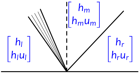
In the figure we have one wave going in each direction, but since the wave speeds depend on $q$ and can have either sign, it is possible to have both waves going left, or both going right.
To solve the Riemann problem, we must find $q_m$. To do so we must find a state that can be connected to $q_l$ by a 1-shock or 1-rarefaction and to $q_r$ by a 2-shock or 2-rarefaction. We must also ensure that the resulting waves satisfy the entropy condition.
Shock waves
Let us now consider a shock wave connecting a known state $q_*=(h_*, h_* u_*)$ to an unknown state $q=(h,hu)$. In the context of the Riemann problem, $q_*$ will be the initial left or right state and $q$ will be the middle state. The Rankine-Hugoniot jump conditions $s(q_r - q_l) = f(q_r) - f(q_l)$ for a shock wave moving at speed $s$ read
\begin{align} s (h_* - h) & = h_* u_* - h u \\ s (h_* u_* - h u) & = h_* u_*^2 - h u^2 + \frac{g}{2}(h_*^2 - h^2). \end{align}It is convenient to define $\alpha = h - h_*$. Then we can combine the two equations above to show that the momenta are related by
\begin{align} \label{SW:hugoniot-locus} h u & = h_* u_* + \alpha \left[u_* \pm \sqrt{gh_* \left(1+\frac{\alpha}{h_*}\right)\left(1+\frac{\alpha}{2h_*}\right)}\right] \end{align}for a shock moving with speed
\begin{align} \label{SW:shock-speed} s & = \frac{h_* u_* - h u}{h_* - h} = u_* \mp \sqrt{gh_* \left(1+\frac{\alpha}{h_*}\right)\left(1+\frac{\alpha}{2h_*}\right)} = u_* \mp \sqrt{gh \frac{h_* + h}{2h_*} } \end{align}Choosing the plus sign in \eqref{SW:hugoniot-locus} (which yields the minus sign in \eqref{SW:shock-speed}) gives a 1-shock. Choosing the minus sign in \eqref{SW:hugoniot-locus} (which yields the plus sign in \eqref{SW:shock-speed}) gives a 2-shock. Notice from the last expression in \eqref{SW:shock-speed} that as $h \to h^*$ the shock speed approaches the corresponding characteristic speed \eqref{SW:char-speeds}, while the ratio of the jumps in momentum and depth approaches that suggested by the eigenvectors \eqref{SW:fjac-evecs}.
We can now consider the set of all possible states $(h, h u)$ satisfying \eqref{SW:hugoniot-locus}. This curve in the $h - hu$ plane is known as the hugoniot locus; there is a family of hugoniot loci for 1-shocks and another for 2-shocks. Below we plot some members of these two families of curves.
%matplotlib inline
import numpy as np
import matplotlib.pyplot as plt
from exact_solvers import shallow_water
from collections import namedtuple
from utils import riemann_tools
from ipywidgets import widgets
from utils.snapshot_widgets import interact
State = namedtuple('State', shallow_water.conserved_variables)
Primitive_State = namedtuple('PrimState', shallow_water.primitive_variables)
plt.style.use('seaborn-talk')
g = 1.
interact(shallow_water.plot_hugoniot_loci,y_axis=widgets.fixed('hu'));
The plot above shows the Hugoniot loci in the $h$-$hu$ plane, the natural phase plane in terms of the two conserved quantities. Note that they all approach the origin as $h \rightarrow 0$. Alternatively, we can plot these same curves in the $h$-$u$ plane:
interact(shallow_water.plot_hugoniot_loci,y_axis=widgets.fixed('u'));
Note that in this plane, the curves in each family are simply vertical translates of one another, and all curves asymptote to $\pm \infty$ as $h \rightarrow 0$.
All-shock Riemann solutions
If we knew a priori that both waves in the Riemann solution were shock waves, we could find $q_m$ by finding the intersection of the 1-Hugoniot locus passing through $q_l$ with the 2-Hugoniot locus passing through $q_r$. The Riemann solution would then consist simply of two discontinuities propagating at the speeds given by \eqref{SW:shock-speed}.
Here is an example for which this is the correct solution.
def c1(q, xi, g=1.):
    "Characteristic speed for shallow water 1-waves."
    h = q[0]
    if h > 0:
        u = q[1]/q[0]
        return u - np.sqrt(g*h)
    else:
        return 0

def c2(q, xi, g=1.):
    "Characteristic speed for shallow water 2-waves."
    h = q[0]
    if h > 0:
        u = q[1]/q[0]
        return u + np.sqrt(g*h)
    else:
        return 0
def make_plot_function(q_l,q_r,g=1.,force_waves=None,extra_lines=None):
    states, speeds, reval, wave_types = \
        shallow_water.exact_riemann_solution(q_l,q_r,g,
                                             force_waves=force_waves)
    def plot_function(t,plot_1_chars=False,plot_2_chars=False):
        ax = riemann_tools.plot_riemann(states,speeds,reval,wave_types,
                                        t=t,t_pointer=0,extra_axes=True,
                                        variable_names=shallow_water.conserved_variables,
                                        fill=[0]);
        if plot_1_chars:
            riemann_tools.plot_characteristics(reval,lambda_1,axes=ax[0],
                                               extra_lines=extra_lines)
        if plot_2_chars:
            riemann_tools.plot_characteristics(reval,lambda_2,axes=ax[0],
                                               extra_lines=extra_lines)
        shallow_water.phase_plane_plot(q_l,q_r,g,ax=ax[3],
                                       force_waves=force_waves,y_axis='u')
        plt.show()
    return plot_function

def plot_riemann_SW(q_l,q_r,g=1.,force_waves=None,extra_lines=None):
    plot_function = make_plot_function(q_l,q_r,g,force_waves,extra_lines)
    interact(plot_function, t=widgets.FloatSlider(value=0.,min=0,max=.9),
             plot_1_chars=Checkbox(description='1-characteristics',
                                   value=False),
             plot_2_chars=Checkbox(description='2-characteristics'))
q_l  = State(Depth = 1.,
             Momentum = 1.)
q_r = State(Depth = 1.,
            Momentum = -1.)

plot_riemann_SW(q_l,q_r)
Check the boxes to plot the characteristic families, and notice that the 1-characteristics impinge on the 1-shock; the 2-characteristics impinge on the 2-shock. Thus these shocks satisfy the entropy condition.
Dam-break problem: all-shock solution
Here's another example, which you might think of as modeling a dam that suddenly breaks. The water is initially at rest on both sides, but much deeper on the left.
q_l  = State(Depth = 4.,
             Momentum = 0.)
q_r = State(Depth = 1.,
            Momentum = 0.)
plot_riemann_SW(q_l,q_r,force_waves='shock',
                extra_lines=[[[0,0],[-1.317,1.]]]);
Check the box to plot the 1-characteristics. Notice that they don't impinge on the 1-shock; instead, characteristics are diverging away from it. This shock does not satisfy the entropy condition and should be replaced with a rarefaction. The corresponding part of the Hugoniot locus is plotted with a dashed line to remind us that it is unphysical.
Now check the box to plot the 2-characteristics. Notice that these do impinge on the 2-shock; this is an entropy-satisfying shock, and the Hugoniot locus is plotted as a solid line.
The entropy condition
To be physically correct, each of these waves must satisfy the Lax entropy condition. Notice that the shock speed \eqref{SW:shock-speed} can be written as
\begin{align} s & = u_* \pm \sqrt{gh \frac{h_* + h}{2h_*} } \end{align}
Thus the 1-shock entropy condition reads
The second expression for the shock speed is obtained by noticing
that the shock speed is invariant under transposition of the left and right states.
The first and second inequalities both simplify to
Similarly, it can be shown that the entropy condition for a 2-shock connecting $q_m$ and $q_r$ is satisfied if and only if
If \eqref{SW:1-entropy} or \eqref{SW:2-entropy} is violated, then the
corresponding wave must be a rarefaction rather than a shock.
Go back and look at the phase plane plots above. You'll notice that the 1-Hugoniot locus passing through $q_\ell$ is plotted with a solid line for $h>h_\ell$ and with a dashed line for $h
Rarefaction waves
Integral curves
In the LWR traffic flow model, we saw that a rarefaction wave consisted of a smoothly-varying density. For the shallow water system, both the depth $h$ and the momentum $hu$ will vary smoothly through a rarefaction wave. A given rarefaction wave is associated with just one characteristic family, and the variation within the wave is at all points proportional to the corresponding eigenvector $r_p$. In other words, all values $\tilde{q}=(h,hu)$ in the rarefaction lie on a curve defined by
\begin{align} \label{SW:gen_ode} \tilde{q}'(\xi) & = r_p(\tilde{q}(\xi)). \end{align}Here $\tilde{q}(\xi)$ is a parameterization of the solution. For the shallow water system, \eqref{SW:gen_ode} reads
\begin{align} h'(\xi) = q_1'(\xi) & = 1 \label{SW:dh} \\ (hu)'(\xi) = q_2'(\xi) & = u \pm \sqrt{gh} = \tilde{q}_2/\tilde{q}_1 - \sqrt{g\tilde{q}_1}, \label{SW:dhu} \end{align}
where we take the minus sign for 1-waves and the plus sign for 2-waves.
We can think of \eqref{SW:dh}-\eqref{SW:dhu} as an initial value ODE;
fixing the value of $\tilde{q}$ at one point in the rarefaction wave
determines the whole solution of \eqref{SW:dh}-\eqref{SW:dhu}. We
refer to each of these solutions as an integral curve.
For the shallow water system, these equations can be integrated exactly. If we fix one point $(h_*, h_*u_*)$ on the curve, the whole integral curve is defined by
\begin{align} hu & = hu_* \pm 2h(\sqrt{gh_*} - \sqrt{gh}). \end{align}
where now the plus sign is for 1-waves and the minus sign for 2-waves.
This can be rewritten as
From \eqref{SW:riemann-invariant} we see that the value $u + 2 \sqrt{gh}$
is constant along any 1-integral curve, while the value $u-2\sqrt{gh}$ is constant along any 2-integral curve. We refer to these quantities as Riemann invariants for the shallow water system:
In other words, the trajectories plotted above are just the level curves of $w_1$ and $w_2$. This allows us to easily plot the integral curves as a contour plot of $w_1$ or $w_2$:
def plot_int_curves(plot_1=True,plot_2=False,y_axis='hu'):
    N = 400
    g = 1.
    if y_axis == 'hu':
        h, hu = np.meshgrid(np.linspace(0.01,3,N),np.linspace(-3,3,N))
        u = hu/h
        yvar = hu
        ylabel = 'momentum (hu)'
    else:
        h, u = np.meshgrid(np.linspace(0.01,3,N),np.linspace(-3,3,N))
        yvar = u
        ylabel = 'velocity (u)'
    w1 = u + 2 * np.sqrt(g*h)
    w2 = u - 2 * np.sqrt(g*h)
    if plot_1:
        clines = np.linspace(-4,6,21)
        plt.contour(h,yvar,w1,clines,colors='coral',linestyles='solid')
    if plot_2:
        clines = np.linspace(-6,4,21)
        plt.contour(h,yvar,w2,clines,colors='maroon',linestyles='solid')

    plt.axis((0,3,-3,3))
    plt.xlabel('depth h')
    plt.ylabel(ylabel)
    plt.title('Integral curves')
    plt.show()

interact(plot_int_curves, y_axis=widgets.fixed('hu'),
         plot_1=widgets.Checkbox(description='1-wave curves',value=True),
         plot_2=widgets.Checkbox(description='2-wave curves'));
We can also plot the integral curves in the $h$--$u$ plane:
interact(plot_int_curves, y_axis=widgets.fixed('u'),
         plot_1=widgets.Checkbox(description='1-wave curves',value=True),
         plot_2=widgets.Checkbox(description='2-wave curves'));
Note that in this plane the integral curves of each family are simply vertical translates of one another due to the form of the functions $w_1$ and $w_2$. Unlike the Hugoniot loci, the integral curves do not asymptote to $\pm\infty$ as $h \rightarrow 0$ and instead approach a finite value.
Comparison of integral curves and Hugoniot loci
You may have noticed that the integral curves look very similar to the Hugoniot loci, especially when plotted in the $h-hu$ plane. Below we emphasize the differences by plotting the curve from each of these families that passes through a specified point. The difference is less noticeable in the $h-hu$ plane since all of the curves approach the origin.
def compare_curves(wave_family=1, h0=1., u0=0., y_axis='u'):
    h = np.linspace(1.e-2,3,400)

    u = shallow_water.integral_curve(h,h0,h0*u0,wave_family,y_axis=y_axis)
    plt.plot(h,u,'b')
    u = shallow_water.hugoniot_locus(h,h0,h0*u0,wave_family,y_axis=y_axis)
    plt.plot(h,u,'r')
    plt.legend(['Integral curve','Hugoniot locus'])
    if y_axis == 'u':
        plt.plot(h0,u0,'ok')
        plt.ylabel('velocity (u)')
    else:
        plt.plot(h0,h0*u0,'ok')
        plt.ylabel('momentum (hu)')
    plt.xlabel('depth h')
    plt.show()

interact(compare_curves,
         wave_family=RadioButtons(options=[1,2],description='Wave family:'),
         y_axis=RadioButtons(options=['u','hu'],description='Vertical axis:'),
         h0=FloatSlider(min=1.e-1,max=3.,value=1.,description='$h_*$'),
         u0=FloatSlider(min=-3,max=3,description='$u_*$'));
Near the point of intersection, the curves are very close; indeed, they must be tangent at this point since their direction is parallel to the corresponding eigenvector there. Far from this point they diverge; for small depths they must diverge greatly, since the Hugoniot locus never reaches $h=0$ at any finite velocity.
The structure of centered rarefaction waves
Rarefactions appearing in the Riemann solution are also similarity solutions; that is they are constant along any ray $\xi=x/t$. For a $p$-rarefaction connecting states $q_\ell$ and $q_r$, the rarefaction thus has the form
\begin{align} q(x,t) & = \begin{cases} q_\ell & \text{if } x/t \le \lambda_p(q_\ell) \\ \tilde{q}(x/t) & \text{if } \lambda_p(q_\ell) \le \lambda_p(q_r) \\ q_r & \text{if } x/t \ge \lambda_p(q_r). \end{cases} \end{align}It remains to be determined how $\tilde{q}$ varies as a function of $x/t$. This can be determined by noting that each solution value $\tilde{q}$ propagates at the characteristic speed $\lambda_p(\tilde{q})$. Letting $\xi=x/t$, this gives us the condition
\begin{align} \label{SW:char-sim} \lambda_p(\tilde{q}(\xi)) = \xi. \end{align}By combining \eqref{SW:char-sim} with the Riemann invariant condition, we can find $\tilde{h}$ and $\tilde{u}$ within the rarefaction. For concreteness, let us consider a 1-rarefaction connecting $q_l$ and $q_m$. Then \eqref{SW:char-sim} reads $\tilde{u} - \sqrt{g\tilde{h}} = \xi$, which simplifies to
\begin{align} \label{SW:char-sim1} \tilde{h} = \frac{(\tilde{u}-\xi)^2}{g}. \end{align}
Meanwhile, the fact that $w_1(\tilde{q})$ is constant means that
Combining \eqref{SW:char-sim1} with \eqref{SW:w1-const}, we find
We see that $h$ varies quadratically through the rarefaction, while $u$ varies linearly.
Connecting states
Suppose we know that the middle state $q_m$ is connected to the left and right states by rarefactions. Then we can find $q_m$ by finding the intersection of the corresponding integral curves. Here is an example for which this is the physically correct solution:
\begin{align} q_l & = \begin{bmatrix} 1 \\ -1 \end{bmatrix} & q_r & = \begin{bmatrix} 1 \\ 1 \end{bmatrix} \end{align}q_l = State(Depth = 1.,
Momentum = -1.)
q_r = State(Depth = 1.,
Momentum = 1.)
plot_riemann_SW(q_l,q_r)
Notice that the segment of each integral curve that connects to states with a smaller depth is plotted as a solid line, while the segment connecting to states with greater depth is plotted with a dashed line. This again is to remind us that states connected by a rarefaction through the solid part are physical (entropy-satisfying), while states connected by the dashed part would be unphysical (entropy-violating).
Try changing the velocities to $(2, -2)$, and notice that the Riemann solution has a state with almost zero depth in the middle. What happens if you use even larger outflow velocities? We'll discuss this later, in the section on dry states.
Dam-break problem: all-rarefaction solution
Next let us revisit the problem from the section above where we found that the all-shock solution was incorrect. This time we'll try to find an all-rarefaction solution.
q_l  = State(Depth = 4.,
             Momentum = 0.)
q_r = State(Depth = 1.,
            Momentum = 0.)
plot_riemann_SW(q_l,q_r,force_waves='raref')
Plot the 2-characteristics and notice that they cross each other within the 2-rarefaction. This means that the solution we constructed is triple-valued and nonsensical as a solution to this one-dimensional conservation law, and so this portion of the solution is omitted in the plots of depth and momentum. In this case a rarefaction wave is not physical and should be replaced with a shock; the corresponding part of the integral curve is hence shown as a dashed line.
The Riemann solution
To determine $q_m$, we need to know whether each of the two waves is a shock or rarefaction, so that we can use the appopriate Hugoniot locus or integral curve. But to determine the nature of each wave, we need to check \eqref{SW:1-entropy} or \eqref{SW:2-entropy}, which requires knowledge of $h_m$. To deal with this we define a piecewise function $\phi_l(h)$ that gives:
- for $h>h_l$, the momentum connected to $q_l$ by a 1-shock;
- for $h
Thus $\phi$ is partly a 1-Hugoniot locus and partly a 1-integral curve; it gives the value of each precisely in the regime where they are physically correct. We can similarly define a function $\phi_r(h)$ related to the 2-Hugoniot locus and 2-integral curve. The middle state depth $h_m$ is the value for which $\phi_l(h) = \phi_r(h)$. This value can be found computationally via a rootfinding algorithm.
Dam-break problem: correct solution
Below we plot (at last) the correct solution to the dam-break problem, involving a 1-rarefaction and a 2-shock. Plot the characteristics and notice how each family behaves correctly with respect to the corresponding wave in the Riemann solution.
q_l  = State(Depth = 4.,
             Momentum = 0.)
q_r = State(Depth = 1.,
            Momentum = 0.)

plot_riemann_SW(q_l,q_r)
Dry states
The approach just described will yield the correct Riemann solution (provided that the rootfinding algorithm converges) in most situations. However, it will fail if the solution involves dry ($h=0$) states.
Dry states
Dry middle state
Sometimes it seems that there is no way to connect a given pair of left and right states via entropy-satisfying shocks or rarefactions. In the cell below we plot only the physically relevant parts of the integral curves and hugoniot loci passing through the left and right states. Both the $h-u$ and $h-hu$ planes are shown. Try to adjust those states to find a combination for which none of the curves intersect.
def connect_states(h_l=1.,u_l=-1.,h_r=1.,u_r=1.):
    q_l = np.array([h_l,h_l*u_l])
    q_r = np.array([h_r,h_r*u_r])
    fig, ax = plt.subplots(1,2,figsize=figsize)
    shallow_water.phase_plane_curves(q_l[0], q_l[1], 'qleft',
                                     wave_family=1,ax=ax[0])
    shallow_water.phase_plane_curves(q_r[0], q_r[1], 'qright',
                                     wave_family=2,ax=ax[0])
    shallow_water.phase_plane_curves(q_l[0], q_l[1], 'qleft',
                                     wave_family=1,y_axis='hu',ax=ax[1])
    shallow_water.phase_plane_curves(q_r[0], q_r[1], 'qright',
                                     wave_family=2,y_axis='hu',ax=ax[1])
    ax[0].set_title('h-u plane'); ax[1].set_title('h-hu plane');
    ax[0].set_xlim(0,3); ax[1].set_xlim(0,3);
    ax[0].set_ylim(-10,10); ax[1].set_ylim(-10,10);
    plt.tight_layout(); plt.show()

interact(connect_states,
         h_l=widgets.FloatSlider(min=0.001,max=2,value=1),
         u_l=widgets.FloatSlider(min=-5,max=5,value=-1),
         h_r=widgets.FloatSlider(min=0.001,max=2,value=1),
         u_r=widgets.FloatSlider(min=-5,max=5,value=1));
You should find that by making the initial states flow sufficiently fast away from each other, there is no intersection in the $h-u$ plane. In the $h-hu$ plane, the integral curves always intersect at the origin. The reason for this ambiguity is that for zero depth it isn't meaningful to assign a velocity. Thus in the $h-u$ plane we could think of the entire $u$-axis as being part of every integral curve. That means that we can always connect the left and right states via an intermediate state with depth $h=0$ (a dry state).
Since the 1-integral curve through $q_l$ reaches $h=0$ at $u = u_l + 2 \sqrt{gh_l}$ and the 2-integral curve reaches $h=0$ at $u=u_r-2\sqrt{gh_r}$, we see that a dry middle state occurs if and only if $u_l + 2 \sqrt{gh_l} < u_r-2\sqrt{gh_r}$.
It is clear in this case that the solution must consist of two centered rarefaction waves, connecting the left and right states to the middle dry state. These centered rarefactions still have the structure derived above; to complete the solution we only need to know the range of centered characteristics included in each rarefaction. This is most conveniently determined by considering the $h-u$ plane. The 1-integral curve passing through $q_l$ is given by $u = u_l + 2(\sqrt{gh_l}-\sqrt{gh_r})$; it reaches a dry state $h=0$ at $u=u_l + 2\sqrt{gh_l}$. Similarly, the 2-integral curve passing through $q_r$ reaches a dry state $h=0$ at $u=u_r - 2\sqrt{gh_r}$. Thus the dry state solution is given by
\begin{align} q(x,t) & = \begin{cases} q_l & \text{if } x/t \le u_l - \sqrt{gh_l} \\ \tilde{q}_\ell & \text{if } u_l - \sqrt{gh_\ell} \le x/t \le u_l+2\sqrt{gh_l} \\ 0 & \text{if } u_l + 2\sqrt{gh_l} \le x/t \le u_r - 2\sqrt{gh_r} \\ \tilde{q}_r & \text{if } u_r - 2\sqrt{gh_r} \le x/t \le u_r+\sqrt{gh_r} \\ q_r & \text{if } x/t \ge u_r + \sqrt{gh_r}, \end{cases} \end{align}
where $\tilde{q}_\ell$ is given by \eqref{SW:1-raref-struct-h}-\eqref{SW:1-raref-struct-u} and $\tilde{q}_r$ is given by a similar expression.
Here's an example of a Riemann problem whose solution involves a dry middle state:
q_l  = State(Depth = 1.,
             Momentum = -3.)
q_r = State(Depth = 1.,
            Momentum = 4.)
plot_riemann_SW(q_l,q_r)
Dry initial states
What if the left or right state in the Riemann problem is dry? In this case, the solution consists only of a rarefaction wave connecting the non-dry state to $h=0$.
q_l  = State(Depth = 1.,
             Momentum = 0.)
q_r = State(Depth = 0.,
            Momentum = 0.)
plot_riemann_SW(q_l,q_r)
Interactive phase plane and solver
In the phase plane image below, the hugoniot loci are plotted in red and the integral curves in blue. The portion of each curve that satisfies the entropy condition is plotted as a solid line, while the entropy-violating parts are plotted as dashed lines. The curves are plotted for both the left and right states. Thus the function $\phi_l$ just described consists of the solid curve (blue and red parts) passing through the left state $q_\ell$; the function $\phi_r$ is the solid curve (blue and red parts) passing through $q_r$. The intersection of these curves is labeled $q_m$. Click here to go to the interactive phase plane. While you're there, be sure to click and drag the dark circles indicating the values of $q_\ell$ and $q_r$ in the top left plot. The time can also be adjusted by dragging the circle in the top right plot.
Finally, the code below generates an interactive widget that shows the solution to the Riemann problem for arbitrary left and right states, including solutions with dry states.
# Unlike javascript version, this works with dry states
def plot_exact_riemann_solution(h_l=3.,u_l=0.,h_r=1.,u_r=0.,t=0.2):
    q_l = shallow_water.primitive_to_conservative(h_l,u_l)
    q_r = shallow_water.primitive_to_conservative(h_r,u_r)

    x = np.linspace(-1.,1.,1000)
    states, speeds, reval, wave_types = \
        shallow_water.exact_riemann_solution(q_l, q_r, grav=g)
    q = reval(x/t)
    primitive = shallow_water.conservative_to_primitive(q[0],q[1])

    fig = plt.figure(figsize=figsize)
    names = shallow_water.primitive_variables
    axes = [0]*len(q_l)
    for i in range(len(q_l)):
        axes[i] = fig.add_subplot(1,len(q_l),i+1)
        q = primitive[i]
        plt.plot(x,q,'-k',linewidth=3)
        if i==0:
            plt.fill_between(x,q,color='b')
        plt.title(names[i])
        qmax = max(q)
        qmin = min(q)
        qdiff = qmax - qmin
        axes[i].set_ylim((qmin-0.1*qdiff,qmax+0.1*qdiff))
        axes[i].set_xlim(-1,1)
    plt.show()

interact(plot_exact_riemann_solution,
         h_l=FloatSlider(min=0.,max=10.,step=0.1,value=3.,
                                 description=r'$h_l$'),
         u_l=FloatSlider(min=-5.,max=5.,step=0.1,value=0.,
                                 description=r'$u_l$'),
         h_r=FloatSlider(min=0.,max=10.,step=0.1,value=1.,
                                 description=r'$h_r$'),
         u_r=FloatSlider(min=-5.,max=5.,step=0.1,value=0.,
                                 description=r'$u_r$'),
         t=(0.1,1.,0.1));